Fundamentals
Closed-loop control of piezo motors: encoder selection, controller architecture, PID tuning
Building servo systems around friction-drive actuators that have no inherent position feedback
Why closed-loop is mandatory
A piezoelectric ultrasonic motor is a friction-drive device. There is no gearing, no leadscrew, and no inherent relationship between the electrical input and the output position. Apply a drive signal and the motor moves; remove it and the motor stops (held in place by static friction). But exactly how far it moves per unit time depends on preload force, temperature, surface condition, load, humidity, and wear. Open-loop position control is, for all practical purposes, impossible.
This is fundamentally different from stepper motors, where each electrical step corresponds to a deterministic angular increment, or voice coil actuators, where current maps linearly to force. Piezo motors demand closed-loop control not as a refinement but as a basic operational requirement. Without a position sensor and a feedback controller, you cannot command a piezo motor to a specific location and trust that it arrives there.
The upside: when closed-loop control is done well, piezo motors deliver positioning performance that is difficult or impossible to achieve with electromagnetic alternatives. Sub-nanometer resolution, sub-microradian angular accuracy, zero backlash, no magnetic field emission, high stiffness at rest, and power-off position holding. The challenge is that the controller must contend with nonlinear friction, resonant dynamics, and parameter variation that make tuning considerably more involved than a standard servo.
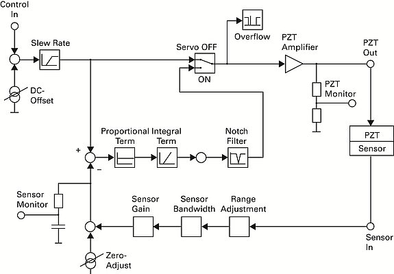
Image: Physik Instrumente (PI)
Encoder technologies for piezo motor systems
The position sensor (encoder) is the foundation of the closed-loop system. Its resolution, accuracy, update rate, and noise floor determine the achievable positioning performance. You cannot servo to a resolution finer than the encoder can resolve.
Optical encoders
Optical encoders use a glass or metal scale with a periodic grating pattern, read by an optical head that generates sinusoidal or digital signals as the scale moves.
Linear optical encoders are the most common feedback sensor for piezo-driven linear stages.
- Incremental encoders produce periodic signals (A and B quadrature channels) that the controller counts to track position changes. They require a reference (homing) operation at startup. Resolution depends on the grating pitch and the interpolation electronics. A 20-micrometer pitch grating with 1000x interpolation yields 20 nm resolution. Top-end systems achieve 1 nm interpolation or better.
- Absolute encoders provide a unique position code at every location. No homing required. Resolution is set by the finest bit of the absolute code. More expensive and bulkier than incremental encoders for the same resolution.
Key specifications for optical encoders in piezo motor applications:
| Parameter | Typical range | Impact on servo |
|---|---|---|
| Resolution | 1 nm to 1 um | Sets minimum step size |
| Accuracy | +-0.1 um to +-5 um over full travel | Limits absolute positioning accuracy |
| Repeatability | +-5 nm to +-100 nm | Determines practical positioning precision |
| Maximum speed | 1 to 5 m/s | Must exceed motor top speed |
| Update rate / bandwidth | 1 MHz to 50 MHz count rate | Must support control loop sample rate |
| Signal period | 4 um to 40 um | Affects interpolation noise |
Common encoder brands in piezoelectric stage applications: Renishaw (RESOLUTE, TONiC), Heidenhain (LIP, LIF series), MicroE / Celera Motion (Mercury, Optira), and Numerik Jena (LIA, LIK series). For nanometer-resolution stages, the Renishaw RESOLUTE (1 nm resolution, absolute) and Heidenhain LIP 382 (2 nm resolution, incremental) are frequently specified.
Installation considerations. Optical encoders require precise mounting to maintain the correct gap (typically 0.5 to 1.5 mm) between the read head and scale. Contamination (dust, oil, condensation) degrades signal quality. In vacuum or cleanroom applications, encoder selection must account for outgassing and particle generation.
Capacitive sensors
Capacitive sensors measure the distance between a probe face and a conductive target by measuring the capacitance of the gap. They are non-contact, have no periodic error, and achieve sub-nanometer resolution.
Strengths for piezo motor applications:
- Resolution to 0.01 nm (in laboratory conditions).
- No periodic error (unlike interpolated optical encoders, which exhibit cyclic error at the grating pitch).
- Absolute measurement (no homing required).
- Excellent linearity over short ranges (typically 10 to 500 um full scale).
Limitations:
- Short measurement range (micrometers to low millimeters). This limits their use to short-travel stages or as secondary sensors in dual-sensor architectures.
- Sensitivity to target flatness, tilt, and material properties.
- Sensitivity to environmental changes (humidity, temperature) affecting the dielectric constant of the gap medium.
- Update rates typically limited to 10 to 100 kHz, sufficient for most servo applications but below what high-speed digital encoders achieve.
Capacitive sensors are the standard choice for nanopositioning stages with travel under 1 mm, where their absolute measurement and sub-nanometer resolution are unmatched. For longer-travel piezo motor stages, optical encoders dominate.
Leading capacitive sensor suppliers: Lion Precision (now part of IDS), Micro-Epsilon (capaNCDT), Physik Instrumente (internal sensors in PI nanopositioning stages).
Interferometric sensors
Laser interferometers measure displacement by counting interference fringes between a reference beam and a measurement beam reflected from a moving target. The fundamental resolution is a fraction of the laser wavelength (typically 633 nm for HeNe, giving a fringe spacing of 316.5 nm before interpolation).
Performance:
- Resolution: 0.01 nm to 1 nm with electronic interpolation.
- Accuracy: limited by the stability of the laser wavelength and the refractive index of the air path. In controlled environments, sub-nm accuracy over millimeters of travel is achievable.
- Range: essentially unlimited (meters of travel) with incremental measurement.
- Update rate: 1 MHz or higher.
Practical challenges:
- Cost: a complete interferometer system (laser source, optics, electronics) costs 10,000 to 50,000 USD, dwarfing the cost of the motor and stage.
- Air path sensitivity: changes in air temperature, pressure, and humidity alter the refractive index and introduce measurement errors. A 1 degree C temperature change causes approximately 1 ppm error (1 nm per mm of measurement range).
- Vibration sensitivity: the optical path must be stable to sub-wavelength levels. Any relative vibration between the optics corrupts the measurement.
- Beam alignment: requires careful optical alignment and mounting.
Interferometers are used in metrology-grade applications (semiconductor lithography, calibration, research) where their accuracy justifies the cost and complexity. For most industrial piezo motor applications, optical encoders provide sufficient performance at a fraction of the cost.
Choosing the right sensor
A practical decision framework:
| Travel range | Resolution target | Recommended sensor |
|---|---|---|
| < 100 um | < 0.1 nm | Capacitive |
| < 1 mm | < 1 nm | Capacitive or interferometer |
| 1 mm to 100 mm | < 10 nm | High-resolution optical encoder |
| 1 mm to 100 mm | < 1 nm | Interferometer |
| > 100 mm | < 100 nm | Optical encoder |
| > 100 mm | < 1 nm | Interferometer (with environmental compensation) |
Image: Physik Instrumente (PI)
Controller architecture
The controller closes the loop between the encoder and the motor drive electronics. Its architecture, update rate, and computational capability directly determine positioning performance.
Analog vs. digital controllers
Analog controllers were common in early piezo motor systems and still appear in simple OEM applications. They use op-amp circuits to implement proportional-integral (PI) or proportional-integral-derivative (PID) compensation. Advantages: zero computational latency, high effective bandwidth. Disadvantages: limited flexibility, no adaptive algorithms, difficult to tune precisely, and aging of analog components causes drift.
Digital controllers dominate modern systems. A digital controller samples the encoder, computes the control law, and outputs a drive command at a fixed update rate. The key specifications are:
- Sample rate: 1 kHz is the minimum for basic positioning. 10 kHz is standard for high-performance stages. 50 to 100 kHz is used in demanding servo applications. The Nyquist criterion requires the sample rate to be at least 2x the desired closed-loop bandwidth, but practical considerations (delay, noise filtering, stability margins) push the requirement to 10x or higher.
- Computational latency: the time between reading the encoder and outputting the drive command. Should be a small fraction of the sample period. Modern DSP-based controllers achieve latencies under 10 microseconds.
- Resolution of the DAC output: the drive command is converted to an analog signal (or PWM) that controls the motor. 16-bit DAC resolution is standard; 20-bit or higher for nanometer-resolution stages.
FPGA-based controllers
For the highest performance, FPGA-based controllers offer sub-microsecond latency and deterministic timing. The control law, encoder interface, and drive signal generation all execute in hardware at clock rates of 50 to 200 MHz. This enables control bandwidths above 10 kHz, which is necessary for rejecting mechanical disturbances in high-precision applications.
Companies like Physik Instrumente (E-727), Aerotech (A3200), and ACS Motion Control (SPiiPlus) offer FPGA-based piezo motor controllers with integrated frequency tracking, PID computation, and advanced feedforward capabilities.
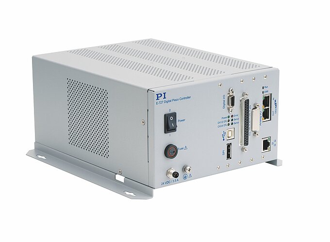
Image: PI E-727 digital piezo controller. The E-727 uses FPGA-based processing for sub-microsecond control loop latency, enabling closed-loop bandwidths above 10 kHz. Source: Physik Instrumente (PI)
The two-loop structure
As discussed in the resonant frequency article, most ultrasonic motor controllers require two nested loops:
-
Resonance tracking (inner loop). This is typically a phase-locked loop (PLL) or admittance-tracking circuit running at or above the drive frequency (e.g., 40 kHz update rate for a 40 kHz motor). Its job is to keep the drive frequency matched to the stator's resonant frequency as it shifts with temperature, load, and aging. This loop is often implemented in analog hardware or FPGA because of the required speed.
-
Position/velocity servo (outer loop). This is the PID (or more advanced) controller that reads the encoder and adjusts the motor's speed command (via drive amplitude, frequency offset, or phase) to achieve the desired position or velocity trajectory. This loop runs at the servo sample rate (1 to 50 kHz typically) and is implemented in a DSP or FPGA.
The separation of these loops simplifies the control design. The inner loop handles the motor's resonant dynamics, presenting the outer loop with a more tractable transfer function (approximately: "the motor's speed is proportional to the commanded amplitude").
PID tuning for friction-drive systems
PID control is the workhorse of positioning systems, but piezo motors present unique challenges that make tuning different from conventional servo systems.
The friction problem
Piezo motors rely on friction between the stator and the moving element (rotor or slider). This friction is the force transmission mechanism, but it is also the primary source of nonlinearity in the control loop.
Static friction (stiction) requires a minimum force to initiate motion. Below this threshold, the motor is locked in place. This creates a dead band in the control loop: small position errors within the stiction zone produce no corrective motion, regardless of the PID gains.
Kinetic friction is typically lower than static friction (the classic Stribeck curve). When the motor breaks free from stiction, it initially accelerates faster than expected because the friction force suddenly drops. This causes overshoot and hunting around the target position.
Velocity-dependent friction varies with speed, often exhibiting a minimum at some intermediate velocity. This makes the motor's transfer function (speed vs. drive amplitude) nonlinear and speed-dependent.
PID tuning strategy
Given these challenges, here is a practical tuning approach:
Step 1: Identify the system. Command a series of step moves at different amplitudes and record the position response. Note the rise time, overshoot, settling time, and any limit-cycle oscillation. Also command constant-velocity moves at different speeds and measure the actual velocity stability.
Step 2: Start with proportional gain (P). Increase P until the system oscillates, then back off to approximately 60% of that value. The Ziegler-Nichols method works as a starting point, but expect to deviate significantly for friction-drive systems.
Step 3: Add integral gain (I). The integral term is essential for eliminating steady-state error and overcoming stiction. Without it, the motor will settle at some offset from the target, held there by static friction with a position error too small to generate enough proportional drive to overcome stiction.
However, integral gain must be managed carefully:
- Anti-windup is mandatory. Without anti-windup, the integrator accumulates during large moves (when the error is saturated) and causes massive overshoot when the motor approaches the target. Clamp the integrator output to a reasonable range.
- Integral gain that is too high causes limit-cycle oscillation. The integrator slowly builds up force, overcomes stiction, the motor lurches, overshoots, and the process repeats. This is the most common failure mode in piezo motor servo tuning.
Step 4: Add derivative gain (D). The derivative term provides damping and reduces overshoot. But it amplifies encoder noise, which can excite the stator's resonance and cause acoustic noise or vibration. Use a low-pass filter on the derivative term (a "filtered derivative" or "D with N filter") to limit high-frequency noise amplification. A typical filter cutoff is 1/10 of the servo sample rate.
Step 5: Address the dead band. Several techniques mitigate stiction dead band:
- Dither. Superimpose a small oscillation on the drive signal when the motor is near the target. This keeps the stator vibrating at low amplitude, preventing full static friction from developing. The dither frequency is typically the motor's resonant frequency at very low amplitude.
- Notch or dead-band compensation. Add a fixed offset to the controller output when it crosses zero, ensuring the minimum drive level always exceeds the stiction threshold. This eliminates the dead band but can introduce noise if implemented crudely.
- Stick-slip stepping. When the position error is within the dead band, command a series of nanometer-scale steps (stick-slip pulses) to walk the motor to the target. This exploits the motor's intrinsic step capability and is very effective for final settling.
Step 6: Tune for each velocity regime. The optimal PID gains at 1 mm/s are different from those at 100 mm/s because the friction characteristics and motor transfer function change with speed. Gain scheduling (switching between pre-tuned gain sets based on commanded velocity or measured speed) improves performance across a wide operating range.
Worked example: tuning a linear piezo stage
Consider a linear stage with 50 mm travel, driven by a traveling-wave ultrasonic motor, with a 5 nm resolution optical encoder, servoed at 10 kHz.
Initial system identification reveals:
- Maximum speed: 250 mm/s
- Stiction dead band: approximately 50 nm
- Rise time (1 mm step): approximately 15 ms
- Natural frequency of stage mechanics: approximately 200 Hz
Tuning steps:
- Set I = 0, D = 0. Increase P until 200 Hz oscillation appears (the stage mechanical resonance is excited). Back off to P = 0.6 * P_critical.
- Add integral gain. Start low, increase until the 50 nm dead band is eliminated (the motor makes final corrections within 100 ms of a step move). Watch for limit cycling; if it appears, reduce I.
- Add derivative gain with a 500 Hz filter. Increase until overshoot on step moves is reduced to < 5% without introducing noise.
- Test at multiple step sizes (100 nm, 1 um, 10 um, 100 um, 1 mm, 10 mm) and velocities (0.1 mm/s, 1 mm/s, 10 mm/s, 100 mm/s). Adjust gains or implement gain scheduling.
- Enable dither at the target position. Set dither amplitude to the minimum that reliably prevents stiction-induced settling error.
Final performance: 20 nm settling accuracy, 30 ms settling time for 1 mm moves, 50 nm position noise at rest.
Feedforward techniques
PID feedback alone is reactive: it corrects errors after they occur. For demanding trajectory-tracking applications, feedforward compensation anticipates the required drive signal and applies it before the error develops.
Velocity feedforward
The simplest and most effective feedforward technique. If you know the motor's speed-vs-drive-amplitude relationship (the "motor curve"), you can compute the approximate drive amplitude needed for any commanded velocity and add it to the PID output. This dramatically reduces tracking error during constant-velocity moves and smooth trajectories.
Implementation: measure the motor curve (drive amplitude vs. actual speed) at several points. Fit a function (often piecewise linear or a low-order polynomial). During motion, compute the feedforward drive amplitude from the commanded velocity and sum it with the PID output.
Acceleration feedforward
For moves with significant acceleration phases, adding a term proportional to commanded acceleration compensates for the motor's inertial lag. The required gain is proportional to the moving mass divided by the motor's force sensitivity (force per unit drive amplitude).
Friction compensation
Model-based friction compensation applies a drive signal specifically to overcome the predicted friction force. The Lugre friction model or the Dahl model can capture the stiction, Coulomb, and viscous friction components. When properly identified and implemented, friction compensation reduces settling time by 30% to 50% compared to PID alone.
Notch filters
If the stage has a lightly damped structural resonance (common in long-travel stages), a notch filter at that frequency prevents the controller from exciting it. Without the notch, increasing PID gains to improve low-frequency performance will eventually excite the resonance and destabilize the loop. The notch filter breaks this trade-off, allowing higher gains below the resonance frequency.
Common failure modes
Limit cycling (hunting)
The motor oscillates back and forth around the target position, never settling. Causes: integral gain too high, stiction too large relative to the encoder resolution, or the controller is alternately driving in one direction and then the other without damping.
Fix: reduce integral gain, add derivative gain with filtering, enable dither, or implement dead-band compensation.
Acoustic noise at rest
The stator emits an audible whine when the motor is "stopped" at a target position. Cause: the servo controller is continuously adjusting the drive signal to maintain position, exciting the stator at or near its resonant frequency.
Fix: reduce controller gains at rest (gain scheduling), allow a small position window within which the controller disables the drive, or reduce the dither amplitude.
Slow final settling
The motor reaches within a few hundred nanometers of the target quickly but takes hundreds of milliseconds to eliminate the last 50 to 100 nm of error. Cause: stiction dead band larger than the controller's minimum effective step size.
Fix: implement stick-slip stepping for final approach, increase dither amplitude, or use a two-stage approach (ultrasonic motor for coarse move, separate piezo stack actuator for fine positioning).
Instability at high gains
Increasing P and D gains destabilizes the system at a specific frequency. Cause: usually a structural resonance of the stage, encoder mount, or coupling between the motor and the load.
Fix: identify the resonance frequency (measure the open-loop frequency response or listen for the oscillation frequency). Apply a notch filter centered on that frequency. If multiple resonances exist, multiple notch filters may be needed.
Overshoot on short moves
Small step moves (< 1 um) overshoot significantly, while larger moves settle cleanly. Cause: the motor's minimum step size is larger than the commanded move. The stiction breakaway is inherently imprecise at the nanometer scale.
Fix: reduce the PID gains for small moves (gain scheduling based on move distance). Use stick-slip mode for sub-micrometer steps. Accept that the motor's effective minimum step size has a practical lower limit, typically 10 to 50 nm for a well-tuned system with a nanometer-resolution encoder.
Controller hardware selection
For production systems, the controller hardware choice depends on performance requirements and volume:
| Controller type | Update rate | Latency | Cost | Typical use case |
|---|---|---|---|---|
| General-purpose MCU (STM32, etc.) | 1 to 10 kHz | 50 to 100 us | $5 to $20 | Low-cost OEM integration |
| DSP (TI C2000, etc.) | 10 to 50 kHz | 5 to 20 us | $10 to $50 | Mid-range motion controllers |
| FPGA (Xilinx, Intel) | 50 to 200 kHz | < 1 us | $50 to $500 | High-performance multi-axis |
| Commercial piezo controller | 10 to 100 kHz | 1 to 10 us | $2,000 to $20,000 | Turnkey integration |
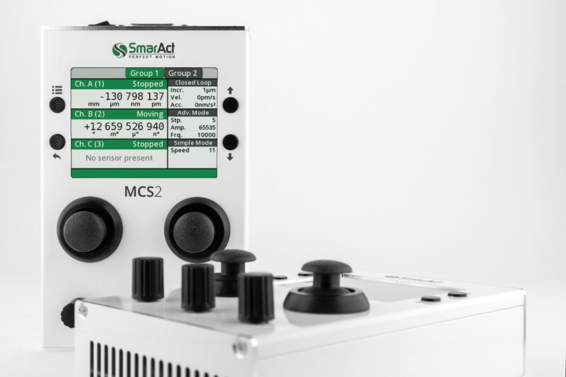
Image: SmarAct MCS2 tabletop controller showing real-time closed-loop position readout in nm/um/mm across multiple axes. The display indicates one axis actively tracking ("Moving") while others hold position ("Stopped"). Source: SmarAct
For prototyping and low-volume applications, commercial controllers from Physik Instrumente, Aerotech, or Newport (MKS) provide the fastest path to a working system. The premium over custom hardware is justified by integrated frequency tracking, tuned PID algorithms, and application support.
For high-volume OEM applications (consumer electronics, automotive, medical devices), custom controller development on a low-cost MCU or DSP is standard practice. The development effort is substantial (6 to 18 months for a production-ready controller) but the per-unit cost reduction is significant at volume.
Summary
Closed-loop control of piezo motors is more demanding than conventional servo design because of the friction-drive mechanism, the resonant stator dynamics, and the nonlinear relationships between drive parameters and motor output. Success requires a high-resolution position sensor matched to the application, a controller architecture with sufficient update rate and computational capability, PID tuning that specifically addresses stiction and the dead-band problem, and feedforward techniques to improve dynamic tracking.
The effort is justified by the result: positioning systems with nanometer resolution, zero backlash, no magnetic emissions, and inherent holding force that electromagnetic alternatives cannot match. The controller is the critical enabler that transforms a friction-drive mechanism into a precision positioning instrument.