Fundamentals
Constant velocity scanning with piezo: why uniformity matters more than peak speed
Velocity ripple, controller bandwidth, and the scanning profiles that determine process quality
In scanning applications, the stage's peak velocity is rarely the specification that determines process quality. What matters is how uniform that velocity remains over the scanning window. A stage capable of 500 mm/s that exhibits ±5% velocity ripple will produce worse results in an inspection (see wafer stage positioning) or coating application than a stage limited to 200 mm/s with ±0.1% ripple. This article examines the sources of velocity non-uniformity in piezo friction-drive stages, the controller architectures that suppress them, and the scanning profiles used to deliver constant velocity over the regions that matter.
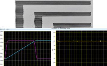
Image: Scan line uniformity (top) versus velocity stability scope trace (bottom) for a PIglide air-bearing stage. Source: Physik Instrumente (PI)
Image: Physik Instrumente (PI)
Why constant velocity matters
Many precision processes are fundamentally rate-sensitive. The exposure energy deposited by a laser onto a moving substrate is proportional to dwell time per unit length, which is inversely proportional to velocity. If the velocity fluctuates by ±3% during a scan, the deposited energy fluctuates by ±3%, producing line-width variation in lithography, thickness variation in coating, or intensity variation in inspection images.
Consider a specific example: a confocal line-scan inspection system acquires pixel rows at a fixed camera trigger rate of 10 kHz. At a nominal scan speed of 100 mm/s, each pixel row corresponds to 10 µm of travel. If the stage velocity drops to 97 mm/s during part of the scan, each pixel row covers only 9.7 µm; if it rises to 103 mm/s, each row covers 10.3 µm. The resulting image is spatially distorted by ±3%, which may or may not be acceptable depending on the measurement tolerance. For critical dimensional metrology, velocity uniformity below ±0.1% is often required.
Sources of velocity ripple in piezo friction-drive stages
Ultrasonic piezoelectric motors drive the stage carriage through a friction contact between a vibrating stator and a moving rail or rotor. This mechanism introduces several sources of velocity non-uniformity.
1. Discrete step structure
The fundamental operating principle of most ultrasonic piezo motors involves generating elliptical motion at the stator tip (see resonant frequency and stator design), which pushes the rotor in discrete micro-steps at the ultrasonic driving frequency (typically 40 to 200 kHz). At low commanded velocities, the stage moves in a series of these micro-steps, each delivering a few nanometres to tens of nanometres of displacement. The resulting velocity waveform contains a periodic ripple at the driving frequency.
At higher velocities, the individual steps blend together because the mechanical bandwidth of the stage (determined by the moving mass and bearing compliance) acts as a low-pass filter. For a stage with a mechanical resonance of 200 Hz and a driving frequency of 100 kHz, the attenuation at the driving frequency is enormous, and the velocity ripple from discrete stepping is negligible. However, at very low scan speeds (below 0.1 mm/s), the step structure can become visible and problematic.
2. Friction variation along the travel
The friction contact between stator and rotor is never perfectly uniform. Surface finish variations, contamination particles, lubricant redistribution, and wear patterns create position-dependent friction modulation. As the stage scans through a region of higher friction, the controller must increase drive amplitude to maintain velocity, and the response time of this adjustment depends on the servo loop bandwidth.
Typical friction variation in a well-maintained piezo stage is ±5% to ±15% of the mean friction force. Without closed-loop velocity control, this would translate directly into ±5% to ±15% velocity variation. The controller must actively compensate.
3. Encoder interpolation artifacts
Optical linear encoders produce sinusoidal signals that are interpolated to generate high-resolution position data. The interpolation process introduces periodic errors (sub-divisional error, or SDE) at the spatial frequency of the encoder grating. When the position signal is differentiated to compute velocity, these periodic position errors become periodic velocity errors.
For an encoder with 4 µm grating pitch and ±20 nm SDE, the velocity error contribution at scan speed v is:
velocity_error = 2π × v × (SDE amplitude) / (grating pitch)
At v = 100 mm/s: velocity_error = 2π × 100 × 20 nm / 4 µm = 2π × 100 × 0.02 / 4 = ±3.14 mm/s
This is ±3.14% of the scan speed, which is significant. The frequency of this ripple is v / pitch = 100 / 0.004 = 25 kHz. Whether this ripple affects the process depends on the application's sensitivity to high-frequency velocity variations.
4. External disturbances
Floor vibrations, cable drag forces, and acoustic disturbances all introduce velocity perturbations. Cable management is particularly important in scanning applications: if the cable bundle connecting the stage exerts a position-dependent drag force, the velocity profile will reflect that force signature. Proper cable routing with low-stiffness cable carriers or cable loops that do not change their drag profile over the scan range is essential.
Controller bandwidth and velocity servo architecture
The stage controller is the primary tool for suppressing velocity ripple. The effectiveness of the controller depends on its architecture, bandwidth, and update rate.
Open-loop velocity control
In the simplest approach, the controller commands a fixed drive amplitude and frequency that, in a nominal friction model, should produce the desired velocity. Any disturbance (friction variation, cable drag, thermal drift) directly perturbs the velocity with no correction. Open-loop velocity uniformity is typically ±5% to ±20%, which is unacceptable for most scanning applications.
Closed-loop position-based velocity control
Most piezo stage controllers implement a position servo loop: the controller reads the encoder, computes the position error, and adjusts the drive signal to minimize position error. For scanning, the controller generates a trajectory (a time-varying position setpoint) and the stage follows it. Velocity is controlled implicitly: if the position profile is a ramp (constant velocity segment), and the stage tracks the ramp with small following error, the velocity is approximately constant.
The velocity uniformity of this approach depends on:
-
Servo bandwidth: the frequency up to which the position loop can track the commanded trajectory. A higher bandwidth loop suppresses disturbances over a wider frequency range. Typical piezo stage position servo bandwidths range from 50 Hz (low-performance) to 2 kHz (high-performance).
-
Following error during constant velocity: during a constant-velocity scan, the following error in a well-tuned PID loop settles to a constant value (determined by the velocity feedforward gain). The velocity error is then dominated by disturbance rejection rather than trajectory tracking.
-
Update rate: the controller's servo update rate (typically 5 kHz to 50 kHz) determines the Nyquist limit for disturbance rejection. Disturbances above half the update rate cannot be corrected.
Velocity feedforward
Adding a velocity feedforward term dramatically improves scanning performance. Instead of relying entirely on the position error signal to drive the stage, the controller injects a drive signal proportional to the commanded velocity. This reduces the position error during constant-velocity segments, which means the position loop has less work to do and can respond more effectively to disturbances.
The feedforward gain is typically calibrated by running the stage at several velocities and measuring the drive signal required to maintain each velocity. A look-up table or linear model maps commanded velocity to feedforward drive amplitude.
With well-tuned velocity feedforward, the following error during constant-velocity scanning can be reduced by 10x to 100x compared to feedback-only control.
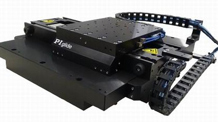
Image: Physik Instrumente (PI)
Dedicated velocity servo loop
The highest-performance scanning stages implement a dedicated velocity feedback loop, in addition to the position loop. The velocity signal is derived from the encoder (using a differentiating filter or a state observer), and a separate controller acts on the velocity error. This dual-loop architecture (inner velocity loop, outer position loop) provides:
- Higher disturbance rejection bandwidth for velocity perturbations
- Better decoupling between position tracking and velocity regulation
- Reduced sensitivity to friction variation
Velocity servo bandwidths of 500 Hz to 3 kHz are achievable, depending on the encoder resolution, the signal processing quality, and the mechanical dynamics of the stage.
Scanning profiles
A scanning application rarely requires constant velocity across the entire travel range. The useful scan window is a subset of the total travel; the remaining travel is used for acceleration, deceleration, and direction reversal. The scanning profile describes the velocity as a function of position (or time) during each scan line.
The trapezoidal profile
The simplest scanning profile is trapezoidal: the stage accelerates at constant acceleration, reaches the scan velocity, maintains that velocity across the scan window, decelerates, and reverses. The key parameters are:
- Scan velocity (v_scan): the constant velocity during the useful scan region
- Acceleration (a): determines how quickly the stage reaches v_scan
- Acceleration distance (d_acc): the travel consumed during acceleration, d_acc = v_scan² / (2a)
- Scan length (L_scan): the useful constant-velocity region
- Turnaround distance (d_turn): the total travel beyond the scan window needed for deceleration, reversal, and re-acceleration. For a symmetric trapezoid, d_turn = 2 × d_acc at each end.
Example: For a scan velocity of 200 mm/s and an acceleration of 2000 mm/s² (≈ 0.2 g), the acceleration distance is 200² / (2 × 2000) = 10 mm. If the scan window is 100 mm, the total stage travel must be at least 100 + 2 × 10 = 120 mm. This means 83% of the travel is usable for scanning; 17% is overhead.
If the scan velocity is increased to 500 mm/s at the same acceleration, the acceleration distance becomes 500² / 4000 = 62.5 mm, and the total travel must be 225 mm (only 44% usable). Higher scan speeds demand either higher acceleration capability or longer total travel, or they reduce the usable scan fraction.
S-curve profiles
Trapezoidal profiles have instantaneous changes in acceleration (infinite jerk) at the transitions between acceleration and constant-velocity segments. These jerk transients excite mechanical resonances in the stage and payload, causing vibration that takes time to damp out. The result is a settling period at the beginning of the constant-velocity segment during which the velocity is not truly constant.
S-curve (or jerk-limited) profiles replace the sharp acceleration transitions with smooth curves, typically third-order polynomials or sinusoidal blends. The jerk (rate of change of acceleration) is limited to a maximum value, and the acceleration ramps smoothly from zero to its peak and back to zero. This eliminates the high-frequency excitation of structural resonances, and the velocity reaches its constant value with less overshoot and ringing.
The trade-off: S-curve profiles require more travel for the acceleration/deceleration phases than trapezoidal profiles at the same peak acceleration and velocity. The acceleration distance increases by approximately 30% to 50% for a sinusoidal jerk profile compared to a constant-acceleration trapezoid.
Bidirectional scanning
Many applications use bidirectional scanning: the stage scans in one direction, reverses, and scans in the opposite direction, covering the same or adjacent region. This doubles the throughput compared to unidirectional scanning (where the return stroke is wasted).
Bidirectional scanning introduces additional challenges:
- Reversal settling: after the deceleration, reversal, and re-acceleration, the velocity must reach the scan speed with sufficient uniformity before the scan window begins. The turnaround time and distance must be budgeted carefully.
- Reversal-dependent errors: friction, bearing preload, and controller dynamics may differ between the two scan directions, causing direction-dependent velocity offsets. The controller must compensate for these asymmetries.
- Data stitching: if the process acquires data during both scan directions, the data from the forward and reverse passes must be registered correctly. Any systematic velocity difference between directions will cause a stitching error.
Trigger-based scanning
Instead of relying on the stage to maintain constant velocity, some systems use encoder-triggered data acquisition. The stage's encoder generates a trigger pulse at fixed position intervals (e.g., every 1 µm), and the camera or sensor acquires data at each trigger. This approach makes the data acquisition synchronous with position rather than time, which inherently compensates for velocity variation: even if the stage velocity fluctuates, each data point corresponds to the same position increment.
However, trigger-based acquisition does not eliminate all effects of velocity variation. If the sensor's integration time is fixed (e.g., a CCD camera with a fixed exposure time), a slower velocity means the stage moves less during the exposure, effectively changing the spatial averaging of each pixel. For dose-sensitive processes (laser writing, coating), the dwell time per unit length changes with velocity regardless of triggering strategy.
Applications requiring uniform scan speed
Optical inspection
Line-scan cameras operating at fixed line rates require constant stage velocity to produce geometrically correct images. Time delay integration (TDI) cameras, commonly used in semiconductor wafer inspection, are particularly sensitive: the TDI operation integrates signal from multiple pixel rows as the image moves across the sensor at a speed matched to the stage velocity. If the stage velocity deviates from the design speed, the TDI integration degrades, causing image blur. The velocity matching requirement for TDI cameras is typically ±0.1% to ±0.5%.
Laser processing
Laser scribing, cutting, and annealing processes deposit energy as the beam traces a path on the workpiece. The energy per unit length is P/v, where P is the laser power and v is the scan velocity. For uniform processing, v must be constant. In display manufacturing, for example, laser lift-off processes require velocity uniformity below ±1% to achieve uniform adhesion release across the panel.
Coating and dispensing
Slot-die coating and inkjet dispensing on moving substrates require constant relative velocity between the coating head and the substrate. Velocity variation produces thickness variation (for slot-die) or drop-spacing variation (for inkjet). In printed electronics, where conductive trace resistance depends on thickness uniformity, velocity ripple directly impacts device performance.
Surface profiling
Contact and non-contact surface profilers (stylus profilometers, white-light interferometers) scan across a surface while measuring height. If the scan velocity varies, the spatial sampling rate changes, affecting the measurement bandwidth and the fidelity of the surface map. For traceable surface roughness measurements (per ISO 4287), the scan speed must be constant to within the instrument's specification, typically ±2% to ±5%.
Quantifying velocity uniformity
Velocity uniformity is specified in several ways, and the choice of metric matters.
Peak velocity error
The simplest metric: the maximum instantaneous velocity deviation from the commanded velocity, expressed as a percentage. Example: ±0.5% of v_scan. This is a worst-case specification.
RMS velocity error
The root-mean-square velocity deviation over the scan window. This weights all deviations equally and is less sensitive to occasional transient spikes. Typically, the RMS velocity error is 3x to 10x smaller than the peak velocity error for a well-controlled stage.
Velocity error spectrum
The frequency content of the velocity error matters. A ±0.5% velocity ripple at 25 kHz (from encoder interpolation) has very different process implications than a ±0.5% ripple at 10 Hz (from low-frequency friction variation). Some applications are insensitive to high-frequency ripple because the process has its own low-pass characteristic (e.g., thermal diffusion during laser processing). Specifying velocity uniformity as a power spectral density (PSD) of velocity error allows the user to evaluate whether the stage's velocity characteristics are compatible with the process bandwidth.
Measurement methods
Measuring velocity uniformity directly is more challenging than measuring position accuracy.
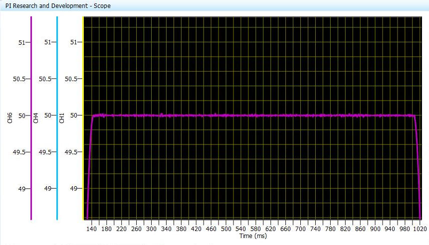
Image: Oscilloscope capture of stage velocity over a constant-velocity scan window. The trace shows sub-0.1% velocity ripple across the full scan duration. Source: Physik Instrumente (PI)
Two approaches are common:
-
Differentiated encoder signal: record the encoder position at a high sample rate (e.g., 100 kHz), then numerically differentiate to obtain velocity. This method captures velocity errors at frequencies up to the Nyquist limit of the sampling rate but is limited by the encoder's own noise and interpolation errors.
-
Laser Doppler vibrometry (LDV): a non-contact velocity measurement with bandwidth exceeding 1 MHz and resolution below 0.01 mm/s. LDV provides a ground-truth velocity measurement independent of the stage's encoder, making it the preferred method for validating velocity specifications.
Controller tuning for scanning performance
Achieving the best scanning velocity uniformity from a given stage requires careful controller tuning, distinct from the tuning used for point-to-point positioning.
Position loop tuning for scanning
For point-to-point positioning, the controller is typically tuned for fast settling with minimal overshoot: high proportional gain, moderate derivative gain, low integral gain. For scanning, the priorities are different:
- Low following error during constant velocity: requires adequate velocity feedforward and sufficient integral gain to eliminate steady-state error.
- Minimal transient at the beginning of the scan window: requires smooth trajectory generation (S-curve profiles) and well-tuned feedforward that matches the actual friction and inertia of the stage.
- High disturbance rejection in the velocity band: requires high servo bandwidth, which in turn requires high controller gains. However, gains must not be so high that they amplify encoder noise or excite structural resonances.
Notch filters and resonance management
Many piezo stages have structural resonances in the 200 Hz to 2 kHz range, depending on the stage size and payload. These resonances limit the achievable servo bandwidth: if the controller gain is increased beyond the point where the loop gain at the resonance frequency exceeds unity, the system becomes unstable. Notch filters (band-reject filters at the resonance frequencies) allow the controller gains to be increased without exciting the resonances, thereby extending the effective servo bandwidth and improving velocity uniformity.
Identifying the resonance frequencies requires a frequency response measurement (swept-sine or noise injection with FFT analysis). The notch filter parameters (centre frequency, bandwidth, depth) must be tuned to match the measured resonances. If the resonance frequency shifts with payload (as it will), the notch filters must be re-tuned after any payload change.
Iterative learning control
For repetitive scanning patterns (the same scan profile executed hundreds or thousands of times), iterative learning control (ILC) can dramatically improve velocity uniformity. ILC records the velocity error from one scan pass and uses it to pre-correct the drive signal on the next pass. Over several iterations, the repeatable components of the velocity error (friction signatures, cable drag profiles, encoder artifacts) are learned and compensated.
ILC can reduce repeatable velocity errors by 10x to 100x, achieving velocity uniformity below ±0.01% for highly repetitive scans. The limitation is that ILC only compensates repeatable errors; random disturbances (vibrations, air currents) are not corrected.
Practical example: budgeting a scan profile
Application: TDI line-scan inspection of 300 mm semiconductor wafers.
Requirements:
- Scan velocity: 250 mm/s
- Velocity uniformity: ±0.2% (required by TDI camera)
- Useful scan length: 300 mm
- Maximum stage travel: 400 mm
Profile design:
Available overhead travel: 400 − 300 = 100 mm, split as 50 mm at each end.
Using an S-curve profile with peak acceleration of 5000 mm/s² (0.5 g) and jerk limit of 200,000 mm/s³:
- Jerk phase duration: t_j = a_max / j_max = 5000 / 200000 = 0.025 s
- Distance during jerk phase: d_j = (1/6) × j_max × t_j³ = (1/6) × 200000 × 0.025³ = 0.52 mm
- Constant acceleration phase: remaining velocity to be gained = 250 − (a_max × t_j) = 250 − 125 = 125 mm/s. Time: t_a = 125 / 5000 = 0.025 s. Distance: d_a = 125 × 0.025 + 0.5 × 5000 × 0.025² = 3.125 + 1.5625 = 4.69 mm
- Second jerk phase: same as first, d_j = 0.52 mm
- Total acceleration distance: 2 × 0.52 + 4.69 = 5.73 mm
This comfortably fits within the 50 mm overhead at each end, leaving 44.27 mm of settling margin after the acceleration phase completes before the scan window begins.
Velocity settling analysis:
After the S-curve acceleration, the dominant velocity perturbation is the residual from the jerk-limited transition, which decays as exp(−t/τ) where τ is the inverse of the velocity loop bandwidth. For a velocity loop bandwidth of 1 kHz (τ = 0.16 ms), the settling to ±0.2% takes approximately 6τ = 1 ms, corresponding to 0.25 mm of travel at 250 mm/s. The 44 mm of margin is more than sufficient.
Velocity error budget during constant-velocity scan:
| Error source | Contribution | Notes |
|---|---|---|
| Friction variation (±10%, compensated by feedforward) | ±0.08% | Assumes 50x disturbance rejection at friction bandwidth |
| Encoder SDE (4 µm pitch, ±15 nm) | ±0.07% | At 250 mm/s, SDE frequency is 62.5 kHz; filtered by mechanics |
| Cable drag variation | ±0.03% | Low-stiffness cable carrier |
| Floor vibration (typical cleanroom, 10 µm/s RMS) | ±0.04% | Passive vibration isolation assumed |
| Controller quantization and latency | ±0.02% | 20 kHz servo rate, 16-bit DAC |
| RSS total | ±0.11% |
The ±0.11% RSS total provides comfortable margin against the ±0.2% requirement.
Summary
Peak scan speed is a marketing number. Velocity uniformity over the scan window is what determines process quality. The primary tools for achieving uniform velocity are controller bandwidth, velocity feedforward, jerk-limited trajectory profiles, and careful mechanical design (low friction variation, good cable management). When evaluating a stage for scanning applications, request the velocity error specification over the scan window, along with the measurement method and conditions. If the vendor cannot provide this data, that itself is informative.