Fundamentals
Multi-axis piezo configurations: stacking, interpolation, and controller architecture
XY and XYZ stage design choices and the controller architectures that make them work
Single-axis positioning is the building block, but most real applications require coordinated motion in two or more degrees of freedom. An XY wafer stage, an XYZ micromanipulator, or a six-axis alignment platform each presents distinct design challenges that go beyond simply bolting two single-axis stages together. The choices made in mechanical architecture, encoder placement, and controller design determine whether a multi-axis system achieves its theoretical performance or falls short by an order of magnitude. This article examines the principal multi-axis configurations used with piezoelectric ultrasonic stages, their trade-offs, and the controller architectures required to realize their potential.
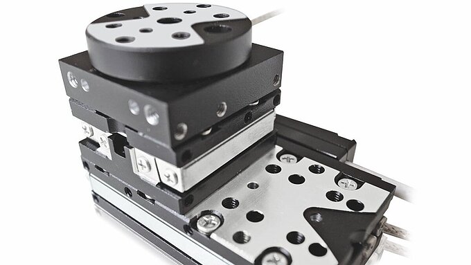
Image: Physik Instrumente (PI)
XY stage design: the fundamental configuration
The XY stage is the most common multi-axis configuration, found in semiconductor inspection, biological microscopy, laser processing, and precision assembly. Two broad mechanical approaches exist: stacked stages and planar (monolithic) stages.
Stacked stages
The simplest XY configuration stacks two single-axis stages orthogonally: the Y stage sits on top of the X stage (or vice versa). The upper stage moves with the lower stage, and the lower stage carries the combined mass of the upper stage plus the payload (see payload mounting for CG offset effects).
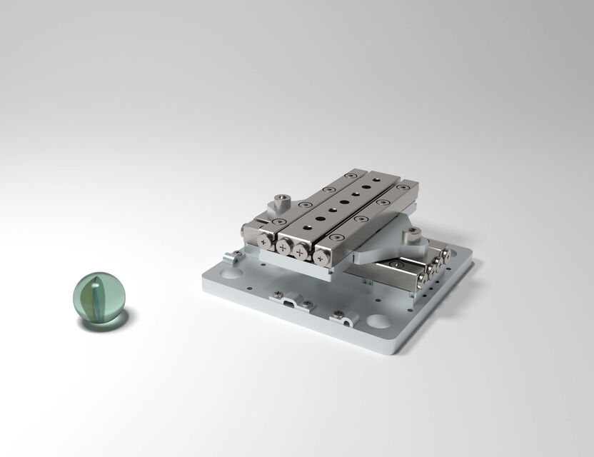
Image: SmarAct XY-SLC-2460 stacked two-axis positioning system. The orthogonal stacking of two linear stages is clearly visible. Source: SmarAct
Advantages:
- Modularity: any two compatible single-axis stages can be combined. This allows the X and Y axes to have different travel ranges, load capacities, or specifications.
- Simplicity: each stage is a self-contained unit with its own encoder, bearings, and drive. No custom mechanical design is needed.
- Cost: stacking standard catalogue stages is less expensive than designing a custom monolithic XY stage.
Disadvantages:
- Asymmetric dynamics: the lower axis carries more mass (upper stage + payload) and therefore has lower resonant frequency and slower dynamic response. The upper axis carries only the payload. This asymmetry means the two axes have different maximum accelerations, settling times, and servo bandwidths. In scanning applications, the slower axis is typically assigned the step-between-scans direction while the faster axis performs the scan.
- Increased height (Z stack-up): the total height of the XY assembly is the sum of both stage heights plus the payload. This raises the payload's centre of gravity and increases the moment arm about the lower stage's bearings, amplifying the effects of acceleration forces on positioning accuracy.
- Cable management complexity: the cables for the upper stage must be routed across the lower stage's moving carriage without introducing drag forces that vary with position.
- Abbe error (discussed in detail below): the vertical offset between the measurement point (typically at the payload surface) and the encoder scale (inside each stage) creates position-dependent angular errors.
Monolithic (planar) XY stages
A monolithic XY stage integrates both axes of motion into a single mechanical structure. The moving carriage translates in both X and Y on a common plane, guided by a two-dimensional bearing system. Two main subtypes exist:
Cross-coupled linear motor stages: two sets of linear motors are arranged orthogonally within a common frame. The carriage is supported by air bearings on a flat reference surface (granite or ceramic). X motion is driven by one set of motors; Y motion by the other. The carriage is the only moving element, so there is no asymmetry between axes.
H-bridge (gantry) stages: for larger travels (hundreds of millimetres), two parallel linear axes (Y1 and Y2) support a crossbeam that carries the X axis. The crossbeam moves in Y; the X carriage moves along the crossbeam in X. This is technically a semi-monolithic design, as the crossbeam is a distinct element.
Advantages of monolithic designs:
- Symmetric dynamics: both axes have similar resonant frequencies and dynamic performance because the moving mass is the same for both directions.
- Low profile: the single-plane design minimizes the Z stack-up, keeping the payload close to the bearing plane and reducing moment loading.
- Reduced Abbe error: encoder scales can be placed at or near the measurement plane.
- Lower moving mass: no axis carries the dead weight of another axis.
Disadvantages:
- Cost and complexity: monolithic XY stages require custom mechanical design, precision machining of the two-axis bearing system, and integrated encoder placement. They are significantly more expensive than stacked stages.
- Fixed aspect ratio: the X and Y travel ranges are determined at design time and cannot be easily changed.
- Air supply requirement: most monolithic XY stages with air bearings require a clean, dry compressed air supply, adding infrastructure cost.
Stacked vs. Monolithic XY Stage Architectures
| Parameter | Stacked | Monolithic/Planar |
|---|---|---|
| Footprint | Larger (two stage widths) | Compact (single platform) |
| Moving mass | Higher (lower axis carries upper) | Lower (single carriage) |
| Crosstalk | Significant (Abbe, cable drag) | Minimal (coplanar motion) |
| Cost | Low (catalogue stages) | High (custom design) |
| Travel range | Flexible (mix and match) | Fixed at design time |
| Flatness / straightness | Limited by bearing stack-up | Superior (air bearing reference) |
| Assembly complexity | Simple (bolt together) | Complex (integrated build) |
Choosing between stacked and monolithic
The decision depends on the application requirements:
| Criterion | Stacked preferred | Monolithic preferred |
|---|---|---|
| Budget | Tight | Flexible |
| Axis asymmetry acceptable | Yes | No |
| Dynamic symmetry required | No | Yes |
| Travel > 200 mm | Either | Yes, for scanning |
| Height constraint | No | Yes |
| Payload CG offset tolerance | Large | Small |
| Production volume | Low (use catalogue stages) | High (justify custom design) |
For most laboratory and R&D applications with moderate performance requirements, stacked stages offer the best value. For high-throughput production tools (semiconductor inspection, display manufacturing), monolithic designs pay for themselves through higher throughput and better accuracy.
Image: Physik Instrumente (PI)
Gantry configurations
Gantry stages are a specific multi-axis topology used when the travel range in one or both axes exceeds what a single-motor stage can efficiently cover, or when the payload must be accessed from below (as in overhead-gantry pick-and-place systems).
The H-bridge gantry
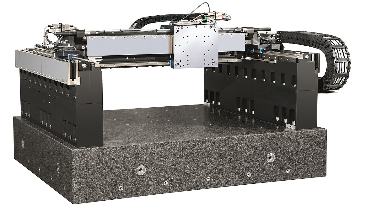
Image: H-bridge gantry stage with dual Y-axis linear motors supporting a crossbeam for the X axis, mounted on a granite base for vibration damping. Source: PI
The most common gantry configuration has two parallel Y-axis rails (Y1 and Y2) separated by a crossbeam that carries the X axis. The Y1 and Y2 carriages move synchronously to translate the crossbeam in Y; the X carriage moves along the crossbeam in X.
Key design considerations:
-
Yaw control: if the Y1 and Y2 carriages do not move in perfect synchrony, the crossbeam rotates about the Z axis (yaw). This yaw error directly corrupts the X-axis position at the payload location. Active yaw control requires independent position feedback on both Y1 and Y2 and a control algorithm that drives both to match. Typical yaw error budgets are below 1 µrad.
-
Crossbeam deflection: the crossbeam acts as a simply supported beam loaded by the X carriage and payload at an arbitrary position along its length. The deflection of the crossbeam varies with the X position, introducing a position-dependent Z error (sag). For a 500 mm crossbeam with a 5 kg payload and a beam cross-section of 40 mm × 60 mm aluminium, the maximum midspan deflection is approximately 2 µm. If Z accuracy matters, this must be calibrated or compensated.
-
Dynamic coupling: accelerating the X carriage exerts a reaction force on the crossbeam, which transmits to the Y1 and Y2 carriages as a disturbance. High servo bandwidth on the Y axes is required to reject this disturbance without introducing Y-position error during X-axis motion.
T-bridge gantry
A simpler variant supports the crossbeam on a single Y-axis carriage at one end and a passive linear guide at the other. This eliminates the yaw synchronization problem but introduces cantilever loading on the Y carriage and more crossbeam deflection. It is used for smaller, lighter payloads where yaw tolerance is less critical.
Image: Physik Instrumente (PI)
Interpolation between axes
In multi-axis systems, the individual axes must work together to produce coordinated motion along arbitrary paths: lines, arcs, spirals, and complex contours. The process of decomposing a desired path into simultaneous axis commands is called interpolation.
Linear interpolation
The simplest form: to move from point A to point B in XY space, the controller commands both axes simultaneously so that the carriage traces a straight line. If the move distance is 10 mm in X and 5 mm in Y, the X axis must move at twice the velocity of the Y axis, and both must start and stop at the same time. The controller generates coordinated velocity profiles (usually trapezoidal or S-curve) for each axis, scaled to ensure simultaneous completion.
Linear interpolation accuracy depends on:
- Trajectory generation synchronization: both axes must receive their position commands at the same time, from the same clock. Any timing skew between axes produces a deviation from the straight-line path.
- Dynamic matching: if the two axes have different servo bandwidths (as in stacked stages), the faster axis will lead the slower axis during acceleration and deceleration, causing a curved deviation from the intended straight line. This is called contouring error.
Circular interpolation
Generating circular arcs requires both axes to follow sinusoidal position profiles (X = R cos θ, Y = R sin θ) with a 90° phase relationship. The accuracy of the resulting circle depends on:
- Gain matching: if the two axes have different position loop gains, the circle becomes an ellipse. A 1% gain mismatch between X and Y produces an ellipticity of approximately 1% (10 µm on a 1 mm radius circle).
- Phase matching: if one axis leads the other by a phase angle δ, the circle becomes an ellipse rotated by δ/2. A phase mismatch of 1° (corresponding to a timing offset of about 28 µs at 100 rev/s) produces measurable ellipticity.
- Reversal spikes: at the 0° and 180° positions (for the X axis) and the 90° and 270° positions (for the Y axis), the axis velocity passes through zero and reverses direction. Friction, bearing preload, and controller dead-zone effects cause small deviations (reversal spikes or quadrant glitches) at these points. Typical magnitudes are 50 nm to 500 nm, depending on the stage quality and controller tuning.
Circular interpolation tests (ISO 230-4, the circular test or ballbar test) are a standard diagnostic for evaluating the coordinated performance of multi-axis systems.
Higher-order interpolation
For complex contours (spline paths, NURBS curves), the controller must generate smooth, jerk-limited trajectories that follow the desired curve while respecting the acceleration and velocity limits of each axis. Modern multi-axis controllers implement real-time spline interpolation with look-ahead algorithms that adjust velocity along the path to ensure the stage can follow the upcoming geometry without exceeding its dynamic limits.
Abbe error and its mitigation
Abbe error (named after Ernst Abbe) is the position error that arises when the measurement point is offset from the measurement axis. It is the dominant geometric error in many multi-axis stage systems, particularly stacked configurations.
The Abbe principle
The Abbe principle states: to avoid first-order measurement error, the measurement axis must be collinear with the axis of the quantity being measured. In practical terms, the encoder scale (measurement axis) should be at the same height and lateral position as the point of interest on the payload.
When this condition is not met, any angular error (pitch, yaw, or roll) of the stage carriage converts to a linear position error at the measurement point through the offset distance.
Quantifying Abbe error
If the measurement point is offset by a distance d from the encoder scale, and the stage carriage has an angular error of α at a given position, the Abbe error is:
ε_Abbe = d × tan(α) ≈ d × α (for small angles, α in radians)
Example: in a stacked XY stage, the payload surface is 80 mm above the X-axis encoder scale. If the X carriage has a pitch error of 5 µrad (a typical value for a well-made cross-roller bearing stage), the Abbe error at the payload is:
ε_Abbe = 80 mm × 5 × 10⁻⁶ = 0.4 µm = 400 nm
This 400 nm error adds directly to the X-axis position error at the payload surface. It is systematic and position-dependent (because the angular error varies with carriage position), but it is not captured by the X-axis encoder because the encoder measures at the scale location, not at the payload.
For a monolithic XY stage with air bearings, the vertical offset between the encoder scale and the payload might be only 10 mm, reducing the Abbe error to 50 nm under the same angular error conditions. This is one of the primary accuracy advantages of monolithic designs.
Abbe error in stacked stages: the compounding problem
In a stacked XY stage, the Abbe error compounds because each axis contributes its own angular errors, and the offset distances are additive:
- The X-axis encoder measures at height z_x (inside the X stage).
- The Y-axis encoder measures at height z_y (inside the Y stage, which sits on top of the X stage).
- The payload is at height z_p (on top of the Y stage).
The total Abbe error in X at the payload is influenced by:
- X carriage pitch error × (z_p − z_x)
- Y carriage roll error × (z_p − z_y) (because Y-axis roll causes X displacement at the payload)
And the total Abbe error in Y at the payload is influenced by:
- Y carriage pitch error × (z_p − z_y)
- X carriage roll error × (z_p − z_x)
The cross-coupling between axes, where roll of one axis affects the in-plane position of the other axis, is a consequence of the stacked geometry and is absent in monolithic designs.
Mitigating Abbe error
Several strategies reduce Abbe error:
-
Minimize the offset distance: use the lowest-profile stages available. Mount the payload as close to the stage as possible. In stacked configurations, place the faster-moving axis on top (closer to the payload) to minimize the offset for the axis that matters most dynamically.
-
Use through-the-workpiece measurement: instead of relying on the stage's internal encoders, measure the payload position directly using an external metrology system (laser interferometer, vision system, or capacitive probe). This eliminates Abbe error entirely because the measurement is made at the point of interest. However, it adds cost and complexity.
-
Calibrate angular errors: measure the stage's pitch, yaw, and roll as a function of position using an autocollimator or laser interferometer angular optics. Then compute the Abbe error at the payload height and apply a position-dependent correction in the controller.
-
Dual-encoder arrangements: some stages mount two linear encoders separated by a known distance in the Abbe-error-sensitive direction. By reading both encoders, the controller can compute the carriage angle and correct for Abbe error in real time. This is common in wafer-stage designs.
Controller architecture for multi-axis systems
The controller is as important as the mechanical stage in determining multi-axis performance. Several architectural approaches exist, with increasing levels of sophistication.
Independent axis controllers
The simplest approach: each axis has its own controller (often a separate hardware unit or a separate control channel), and coordination is handled at a higher level by the host computer. The host sends position commands to each axis, and each controller independently servos its axis.
Limitations:
- Timing skew: if the host sends commands to the X controller and then to the Y controller via sequential communication (e.g., serial commands), there is a time delay between the X and Y commands. At a scan speed of 100 mm/s, a 1 ms delay produces a 100 µm position offset between axes.
- No cross-coupling compensation: each axis controller is unaware of the other axis. It cannot compensate for dynamic interactions (e.g., X-axis reaction forces disturbing the Y axis in a gantry) or geometric coupling (e.g., Abbe error).
- Limited interpolation quality: the host must generate the interpolated trajectory and send it as a stream of discrete points. The controller's ability to follow complex paths is limited by the communication bandwidth.
Synchronized multi-axis controllers
A synchronized controller handles all axes within a single control loop, updated at the same instant by a common clock. This eliminates timing skew and enables true coordinated motion.
Features of a well-designed multi-axis piezo controller:
-
Common time base: all axes read their encoders and update their drive signals at the same instant, typically every 20 to 200 µs (5 to 50 kHz update rate).
-
Coordinated trajectory generator: the trajectory for all axes is computed in a single module, ensuring geometric consistency. The trajectory generator can implement linear, circular, and spline interpolation natively.
-
Cross-axis feedforward and decoupling: the controller can apply corrections for known interactions between axes. For example, in a gantry stage, the controller can feed forward a compensation force to the Y axes proportional to the X-axis acceleration, anticipating the reaction force.
-
Multi-axis error mapping: the controller can store and apply a multi-dimensional calibration map. Instead of correcting X and Y errors independently, the map corrects X error as a function of both X and Y position (and vice versa), capturing geometric errors like orthogonality, straightness, and rotation.
Cascaded control loops
High-performance multi-axis controllers often use cascaded loop structures for each axis:
- Inner current loop (if applicable): controls the drive current to the piezo motor, with bandwidth in the tens of kHz.
- Velocity loop: controls the axis velocity using differentiated encoder feedback, with bandwidth of 500 Hz to 3 kHz.
- Position loop: controls the axis position using encoder feedback, with bandwidth of 50 Hz to 1 kHz.
The cascaded structure allows each loop to handle the dynamics at its own frequency range, providing better overall performance than a single PID loop from encoder to drive signal.
Real-time communication buses
Multi-axis systems with distributed hardware (separate drive amplifiers per axis, remote encoder interfaces) require a real-time communication bus to maintain synchronization. Common buses include:
- EtherCAT: 100 Mbit/s Ethernet-based protocol with cycle times down to 62.5 µs (16 kHz). Widely used in industrial multi-axis systems.
- MACRO (Motion and Control Ring Optical): a fiber-optic ring protocol used in precision stage controllers (notably Delta Tau / Omron), with cycle times as low as 50 µs.
- AXI/SPI internal buses: for compact, integrated controllers where all channels are on the same circuit board, internal bus latency is negligible (sub-microsecond).
The bus cycle time sets the upper limit on the servo update rate for distributed systems. A 100 µs bus cycle (10 kHz) limits the achievable servo bandwidth to approximately 1 to 2 kHz (a practical rule of thumb is that servo bandwidth can be up to 1/5 to 1/10 of the servo update rate for stable operation).
Worked example: specifying a multi-axis system for die bonding
Application: pick-and-place die bonding. An XYZ system picks semiconductor die from a wafer and places them on a substrate with ±5 µm placement accuracy.
Requirements:
- XY travel: 300 mm × 300 mm
- Z travel: 25 mm
- Placement accuracy: ±5 µm (X, Y)
- Throughput: 2 placements per second (500 ms per cycle, including move and settle)
Architecture selection:
The ±5 µm accuracy requirement and the 300 mm travel suggest a gantry configuration:
- Two parallel Y axes (Y1, Y2) with 300 mm travel, supporting a crossbeam
- One X axis on the crossbeam with 300 mm travel
- One Z axis on the X carriage with 25 mm travel
The gantry avoids stacking a 300 mm X stage on a 300 mm Y stage, which would create a very tall assembly with large Abbe error.
Abbe error budget:
The Z height from the Y encoder to the bonding tool is approximately 150 mm (crossbeam height + X stage + Z stage + tool). With a Y-axis pitch error of 3 µrad/mm × 300 mm = 900 µrad maximum over travel (a poor stage), the worst-case Abbe error would be 150 mm × 900 × 10⁻⁶ = 135 µm, which is far too large.
With a high-quality Y axis (pitch error < 5 µrad over full travel), the Abbe error is 150 × 5 × 10⁻⁶ = 0.75 µm, which is acceptable within the ±5 µm budget.
Controller requirements:
- Synchronized 4-axis controller (Y1, Y2, X, Z) with common time base
- Gantry yaw control: Y1 and Y2 driven synchronously with active yaw error correction
- Settling time budget: for a 100 mm move at 1000 mm/s with 10,000 mm/s² acceleration, the move time is approximately 110 ms; the remaining 390 ms is available for settling to ±5 µm, which is easily achievable with a well-tuned controller (typical settling to ±5 µm takes 20 to 100 ms for a piezo stage).
Orthogonality and geometric calibration
In any multi-axis system, the mechanical axes are never perfectly orthogonal. A typical as-built orthogonality error for a high-quality stage is 5 to 50 µrad (1 to 10 arcseconds). For a 300 mm travel, a 20 µrad orthogonality error produces a 6 µm position error at the far corner of the XY field.
Geometric calibration measures and corrects for:
- Orthogonality error: the angle between the X and Y mechanical axes deviates from 90°.
- Straightness error: each axis deviates laterally as it travels. X-axis straightness means the Y position varies as the X carriage moves.
- Scale error: the effective encoder pitch differs slightly between axes.
- Rotation of the coordinate frame: the stage's XY axes are rotated relative to the workpiece coordinate frame.
Calibration is performed using a grid artifact (a plate with a calibrated array of marks) or a pair of laser interferometers measuring X and Y simultaneously. The resulting error map is applied as a 2D correction: for any commanded (X, Y), the controller drives to (X + ΔX(X,Y), Y + ΔY(X,Y)), where ΔX and ΔY are interpolated from the calibration map.
For a 300 mm × 300 mm stage calibrated at a 10 mm grid, the correction map contains approximately 900 points per axis (1800 total). Modern controllers store and interpolate these maps in real time with negligible computational overhead.
Summary
Multi-axis piezo stage design is a system-level problem. The mechanical configuration (stacked, monolithic, gantry) determines the envelope of achievable performance; the controller architecture (independent, synchronized, cascaded) determines how much of that envelope is realized. Abbe error is the dominant geometric error source in stacked systems and must be addressed through design, calibration, or both. Interpolation quality depends on timing synchronization and dynamic matching between axes. When specifying a multi-axis system, treat the controller as a first-class component, not an afterthought. A superior mechanical stage with a mediocre controller will be outperformed by a modest stage with a well-designed, synchronized multi-axis controller.