Repeatability vs. absolute accuracy in piezo stage selection

Every piezo stage datasheet carries two positioning specifications that look similar but describe fundamentally different capabilities: repeatability and absolute accuracy. Confusing them is one of the most common and expensive mistakes in precision motion system selection. The specifications explained article covers how these numbers appear on datasheets. A stage with 50 nm repeatability and 1 µm absolute accuracy is not "worse" than one with 200 nm repeatability and 200 nm absolute accuracy; the two stages are suited to entirely different classes of work. Understanding what each number means, how it is measured, and which one dominates your error budget is the first step toward selecting the right stage for any precision application.

Image: Physik Instrumente (PI)

Definitions: what the numbers actually mean

Repeatability (also called unidirectional repeatability or precision) quantifies how closely a stage returns to the same commanded position across multiple attempts, all approaching from the same direction. It is a measure of random scatter. If you command a stage to move to 10.000 mm twenty times from the same starting direction, the standard deviation of the actual arrived positions is the repeatability. Datasheets typically report it as ±2σ or ±3σ of that distribution.

Absolute accuracy (sometimes called simply accuracy, or trueness in metrology standards) quantifies how closely the stage's reported position matches a traceable reference standard across the entire travel range. It is a measure of systematic error. If the stage's encoder (as discussed in closed-loop control) says the carriage is at 10.000 mm but a laser interferometer says it is actually at 10.000 47 mm, the absolute accuracy error at that point is 470 nm.

The distinction maps directly to the classic metrology concepts of precision versus trueness. A stage can be highly repeatable (tight grouping) while having poor absolute accuracy (the group centre is offset from truth). Conversely, a stage can have excellent absolute accuracy on average yet poor repeatability if the scatter is large around each commanded position.

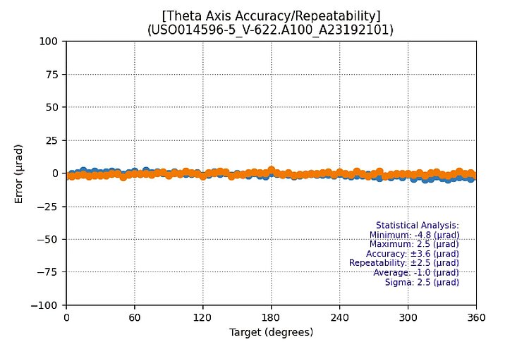
Image: Physik Instrumente (PI)

ISO 230-2 and the formal framework

The international standard ISO 230-2 provides a rigorous framework for evaluating positioning accuracy of machine tool axes, and many piezo stage manufacturers adapt its methodology. Under this standard, each target position is approached multiple times from both directions. The resulting data yields:

• Unidirectional repeatability at each target position (scatter from one direction)
• Bidirectional repeatability at each target position (scatter including reversal error)
• Unidirectional systematic positional deviation (the mean error at each position, one direction)
• Bidirectional accuracy (the full envelope of mean error plus scatter, both directions)

When a datasheet reports a single "repeatability" number, it is usually the worst-case unidirectional repeatability across all measured target positions. When it reports "accuracy," it is usually the maximum bidirectional systematic deviation, sometimes with scatter folded in. Always check the footnotes.

How encoder quality determines repeatability

Repeatability in a closed-loop piezo stage is dominated by the feedback sensor's noise floor and the controller's ability to servo against that noise. The stage structure (bearings, flexures, motor) sets the mechanical limits, but the encoder is almost always the binding constraint on repeatability.

Linear encoder architectures

Three encoder types are common in piezo stages:

1. Optical incremental encoders with interpolated sinusoidal signals. A glass scale with a grating period of 4 µm or 20 µm is read by a scanning head that produces sine and cosine signals. Electronics interpolate these signals, typically by factors of 100x to 4096x, yielding nominal resolutions from 1 nm to 50 nm. The repeatability floor is set by interpolation nonlinearity (sub-divisional error, or SDE), typically 1% to 3% of the grating period. For a 4 µm pitch scale with 1% SDE, the cyclic error component is approximately 40 nm peak-to-peak.

2. Optical absolute encoders, which add a coarse track (or a pseudorandom binary code) so the stage knows its position immediately on power-up without a reference run. The fine-track performance is similar to incremental encoders. The advantage is operational: no homing routine, and no risk of losing position if power is interrupted.

3. Capacitive sensors (sometimes called capacitance gauges). These measure the gap between a target plate and a sensor probe with sub-nanometre noise floors. They are common in short-travel flexure-guided stages (travel under 1 mm). Because there is no periodic scale, there is no sub-divisional error, and repeatability can reach below 1 nm. The limitation is range: capacitance sensors become impractical beyond a few millimetres of travel.

Noise, bandwidth, and the repeatability floor

A typical high-quality optical encoder system in a piezo stage has an electrical noise floor of 0.5 to 2 nm RMS when the stage is stationary. But this number only tells part of the story. The closed-loop servo bandwidth determines how much of that noise translates into actual position jitter. A controller with 1 kHz servo bandwidth will track noise components below 1 kHz, meaning the carriage physically moves in response to low-frequency encoder noise. Higher-frequency noise is attenuated by the mechanical system's mass and stiffness.

Practical repeatability in a well-tuned piezo stage with an optical encoder (4 µm pitch, 1000x interpolation) typically lands between 10 nm and 100 nm, depending on the interpolation quality, the servo tuning, and the thermal environment.

For capacitive-sensor-based flexure stages, repeatability values of 0.5 nm to 5 nm are achievable, though only over short travel ranges (typically under 500 µm).

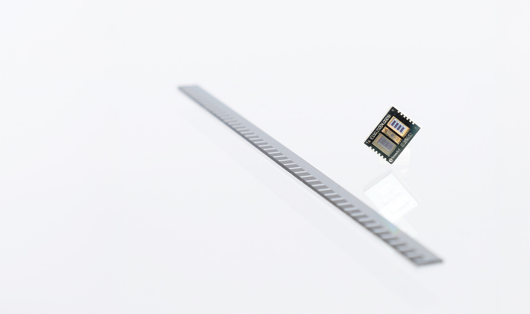
Image: SmarAct GmbH

Environmental vibration and repeatability measurement

Repeatability specifications on datasheets are measured in controlled environments: temperature-stable labs, vibration-isolated optical tables, and low-acoustic-noise rooms. Real installations rarely match these conditions. Understanding how environmental factors inflate the observed repeatability helps predict actual system performance.

Floor vibration coupling

A stage installed on a factory floor experiences vibrations from foot traffic, HVAC systems, and nearby machinery. Floor vibration amplitudes of 0.5 to 5 µm at frequencies of 5 to 50 Hz are common in light industrial environments. The stage's vibration isolation (if any) attenuates these disturbances, but residual vibration at the encoder head adds directly to the measured position scatter.

For a stage with 20 nm datasheet repeatability (3σ), installing it on a floor with 50 nm of vibration at 10 Hz degrades the observed repeatability to approximately √(20² + 50²) = 54 nm, nearly 3x worse than the datasheet. This is not a deficiency of the stage; it is an environmental contribution that the stage cannot reject without active vibration cancellation.

Acoustic coupling

In cleanroom environments, acoustic noise from laminar flow units (typically 65 to 75 dBA) can couple into lightweight stage structures and add 1 to 10 nm of position noise at frequencies of 100 to 500 Hz. This effect is most pronounced for stages with large exposed surface areas and low structural damping.

For applications requiring repeatability below 10 nm, the stage should be enclosed in an acoustic shield or installed in a low-noise environment. Alternatively, a high-bandwidth closed-loop servo can actively reject acoustic disturbances within its control bandwidth.

Thermal cycling during measurement

Even in nominally stable environments, diurnal temperature cycles of 0.5 to 2 °C cause the encoder scale and stage body to expand and contract. If repeatability is measured over a period spanning a temperature cycle, the thermal drift inflates the scatter. A 0.5 °C change in a 100 mm aluminium stage with a glass encoder produces approximately 0.7 µm of differential expansion (as calculated in the thermal drift section below). This appears as a slow drift in the repeated position measurements, increasing the observed repeatability if the measurement period exceeds the thermal time constant of the stage.

Best practice: measure repeatability over a time period shorter than the stage's thermal time constant (typically 15 to 60 minutes), or in an environment controlled to ±0.1 °C.

Calibration methods for absolute accuracy

While repeatability is largely a function of the encoder and servo loop, absolute accuracy depends on how well the entire position-reporting chain has been calibrated against a traceable reference.

Error mapping with a laser interferometer

The gold standard for calibrating a linear stage is comparison against a heterodyne laser interferometer (such as a Renishaw XL-80 or Keysight 5530). The procedure is straightforward:

1. Mount the interferometer optics so the measurement beam is coaxial with the stage's axis of travel.
2. Command the stage to a series of target positions across its full travel (for a 100 mm stage, positions every 1 mm or 0.5 mm are typical).
3. At each target position, record both the stage encoder reading and the interferometer reading.
4. Compute the error at each point: E(x) = encoder_reading(x) − interferometer_reading(x).
5. Fit a correction polynomial or store a look-up table (LUT) of errors.

The correction is then applied in real time by the controller: when the user commands position X, the controller actually drives to X + correction(X). This process is called error mapping or calibration.

A single-pass calibration at 20 °C can reduce the systematic accuracy error of a well-made stage from several micrometres down to 100 to 300 nm across 100 mm of travel. The residual error after calibration is limited by:

• Interpolation nonlinearity (SDE), which repeats every grating period
• Thermal expansion between calibration and measurement
• Mechanical hysteresis or reversal error not captured in the calibration
• Cosine error if the interferometer beam was not perfectly aligned to the stage axis

Higher-order calibration

For applications demanding the highest absolute accuracy (below 100 nm over tens of millimetres), more elaborate calibration strategies are used:

• Bidirectional calibration: separate error maps for positive-direction and negative-direction approaches, with the controller selecting the appropriate map based on the direction of travel.
• Temperature-compensated calibration: embedding a temperature sensor in the stage body and applying a thermal correction model. For an aluminium-bodied stage with a coefficient of thermal expansion (CTE) of 23 µm/(m·K), a 1 °C temperature change causes 2.3 µm of expansion over 100 mm of travel.
• Periodic error correction: mapping the sub-divisional error of the encoder by using the interferometer at very fine position increments (sub-micrometre) and applying a cyclic correction.

Thermal drift: the hidden accuracy killer

Thermal effects are the largest single contributor to absolute accuracy error in most real installations. A calibration performed at 20.0 °C is valid only at that temperature. In practice, the stage body, the encoder scale, and the workpiece all expand or contract as temperature changes.

Quantifying thermal drift

Consider a 150 mm travel aluminium stage with a glass encoder scale. The CTE of aluminium is approximately 23 µm/(m·K); the CTE of glass (soda lime) is approximately 9 µm/(m·K). If the stage body heats by 0.5 °C relative to the calibration temperature:

• Stage body expansion: 150 mm × 23 × 10⁻⁶ /K × 0.5 K = 1.725 µm
• Glass scale expansion: 150 mm × 9 × 10⁻⁶ /K × 0.5 K = 0.675 µm
• Differential expansion (the error): 1.725 − 0.675 = 1.05 µm

This 1.05 µm error appears as a position-dependent accuracy offset that grows linearly with distance from the scale's anchoring point. For applications requiring sub-micrometre absolute accuracy, this is significant.

Mitigation strategies

• Low-CTE scale materials: Zerodur (CTE ≈ 0.05 µm/(m·K)) or Invar scale substrates reduce the scale's thermal sensitivity by orders of magnitude. Some manufacturers offer Zerodur scale options for their highest-accuracy stages.
• Temperature-controlled environments: semiconductor fabs and metrology labs typically hold temperature to ±0.1 °C or better, reducing thermal drift to tens of nanometres.
• Real-time thermal compensation: a temperature sensor on the stage body, combined with known CTE values, allows the controller to apply a correction. This is effective for slow, monotonic temperature drifts but cannot compensate for rapid transients or thermal gradients across the stage.
• Symmetric thermal design: using materials with matched CTEs for the stage body and the scale, or designing the stage so that thermal expansion is symmetric about the measurement axis and cancels out.

What matters more: repeatability or accuracy?

The answer depends entirely on the application. Here is a practical framework:

Repeatability-dominant applications

These applications involve returning to the same set of positions many times, and the absolute location of those positions matters less than the consistency of arrival. Examples:

• Semiconductor wafer inspection: the stage visits the same die sites repeatedly. If every visit lands within ±30 nm of the same spot, the inspection images overlay correctly, even if the "true" position of each site is offset by 500 nm from the nominal coordinate.
• Fiber-optic alignment: once peak coupling is found, the stage must return to that position reliably after perturbations. Absolute position relative to a coordinate frame is irrelevant; return-to-position consistency is everything.
• Repeated dispensing patterns: if a microdispensing system deposits material at the same relative positions on each substrate, repeatability determines pattern fidelity.

For these applications, prioritize encoder quality (low noise, low SDE), servo stiffness, and thermal stability of the encoder mounting. Calibration against an external reference may not be necessary.

Accuracy-dominant applications

These applications require positions to match a coordinate system defined outside the stage. Examples:

• Photomask writing: pattern features must be placed at coordinates matching the design database to within tight tolerances (often below 50 nm). The stage must know where it is in absolute terms, not just return to the same place.
• Multi-tool coordinate transfer: if a workpiece is measured on one stage and then processed on another, the coordinate systems must agree. This requires both stages to have good absolute accuracy relative to a shared reference.
• Metrology instruments: a surface profiler that reports feature positions must have calibrated absolute accuracy; otherwise the reported coordinates of surface features are systematically wrong.

For these applications, invest in high-quality calibration (preferably bidirectional, temperature-compensated), and select stages with low thermal drift and high-quality encoder scales.

Applications where both matter

Some applications require both tight repeatability and good absolute accuracy. Semiconductor lithography (wafer steppers) is the canonical example: the stage must place each exposure field at the correct absolute location on the wafer (accuracy) and must overlay successive exposure layers with nanometre-level consistency (repeatability). These systems use laser interferometer feedback (not encoder scales), active thermal control, and sophisticated error mapping to achieve single-digit-nanometre performance on both metrics simultaneously, at extraordinary cost.

Worked example 1: selecting a stage for a wafer inspection tool

Requirements:

• Travel: 200 mm × 200 mm (XY)
• Stage revisits the same 500 die positions per wafer, imaging each site with a 50x objective (field of view ≈ 250 µm)
• Overlay tolerance between repeat visits: ±100 nm
• Absolute position tolerance (die to coordinate frame): ±5 µm (loose; the vision system performs local alignment)

Analysis:

The critical specification is repeatability, not absolute accuracy. The vision system's local alignment can absorb several micrometres of absolute error, but if the stage does not return to within ±100 nm, the inspection images from successive passes will not register correctly.

Select a stage with:

• Unidirectional repeatability ≤ ±50 nm (providing margin against the 100 nm requirement)
• Optical linear encoders with SDE ≤ 40 nm peak-to-peak
• Servo bandwidth ≥ 500 Hz to maintain repeatability during dynamic settling

Absolute accuracy specification can be relaxed. A stage with ±2 µm absolute accuracy (uncalibrated) is perfectly adequate if the repeatability meets the target.

Cost implication: this stage does not require expensive laser-interferometer calibration or Zerodur encoder scales. A well-made optical encoder stage with standard calibration is sufficient.

Worked example 2: selecting a stage for a photomask metrology system

Requirements:

• Travel: 150 mm × 150 mm
• Measurement positions are defined by the mask design database in an absolute coordinate frame
• Position accuracy requirement: ±100 nm across full travel
• Repeatability requirement: ±50 nm (for averaging multiple measurements)

Analysis:

Both specifications are stringent. The ±100 nm absolute accuracy requirement across 150 mm of travel means that thermal drift alone can consume the entire error budget (recall the 1.05 µm drift per 0.5 °C calculated earlier).

Select a stage with:

• Laser interferometer feedback (not encoder scale), eliminating SDE and scale thermal expansion
• Temperature-controlled environment (±0.1 °C or better)
• Bidirectional error mapping against a traceable reference
• Stage body material with low CTE (granite or Invar base)
• Air bearing guideways (eliminating friction-induced hysteresis)

If a laser interferometer is not practical, select a stage with:

• Zerodur encoder scale (CTE < 0.1 µm/(m·K))
• Bidirectional calibration at operating temperature
• Periodic error correction for SDE
• Temperature sensor and real-time thermal compensation

Cost implication: this system will cost 5 to 20 times more than the inspection stage in Example 1. The accuracy requirement drives the cost.

Worked example 3: repeatability error budget breakdown

Consider a stage with the following specifications:

• Encoder: optical, 4 µm pitch, 4096x interpolation (nominal resolution ≈ 1 nm)
• SDE: ±20 nm (peak-to-peak cyclic error)
• Encoder electrical noise: 1 nm RMS
• Servo bandwidth: 800 Hz

Repeatability error budget:

Error source	Contribution (1σ)	Notes
Encoder noise (electrical)	1.0 nm	Directly measured
SDE (cyclic, treated as random over many positions)	~5.7 nm	≈ 20 nm p-p / (2√3) for uniform distribution
Servo following error (at rest)	0.5 nm	Well-tuned, low disturbance
Thermal encoder drift (short-term, ±0.01 °C)	0.56 nm	Differential expansion of Al stage vs glass scale: 4 mm × (23−9) × 10⁻⁶/K × 0.01 K
Bearing friction hysteresis	2.0 nm	Typical for cross-roller bearings
RSS total (1σ)	~6.1 nm
Repeatability (±3σ)	±18 nm

This budget shows that the SDE of the optical encoder is the dominant contributor. Upgrading to a higher-quality interpolation system (reducing SDE from ±20 nm to ±5 nm) would reduce the total repeatability to approximately ±10 nm (3σ).

Reversal error (bidirectional repeatability)

The discussion above focuses on unidirectional repeatability, where the stage always approaches the target from the same direction. In practice, many applications require bidirectional positioning: the stage moves to targets in arbitrary order, sometimes approaching from the positive direction and sometimes from the negative direction.

The additional error introduced by direction reversal is called reversal error (or backlash, though this term is misleading for piezo stages, which have no gear backlash). In friction-drive piezo stages, reversal error arises from:

• Pre-travel of the friction contact: when the drive direction reverses, the rotor must overcome static friction and elastic compliance in the contact before the stator motion translates into carriage motion. This creates a dead zone, typically 10 to 100 nm.
• Bearing preload asymmetry: cross-roller or ball bearings have slight asymmetry in their restoring forces depending on the direction of load application.
• Controller overshoot: if the servo loop is tuned aggressively, the approach dynamics differ depending on direction.

Bidirectional repeatability is always worse than unidirectional repeatability. Typical values: if unidirectional repeatability is ±20 nm, bidirectional repeatability might be ±40 to ±80 nm. This is an important specification for applications where the stage must approach targets from arbitrary directions, such as point-to-point positioning in a pick-and-place system.

Abbe error: the geometry of measurement

One of the most overlooked contributors to absolute accuracy is Abbe error, named after Ernst Abbe. Abbe error arises whenever the measurement axis does not coincide with the axis of interest. If the encoder measures position at one location on the stage, but the workpiece or tool is at a different location (offset from the encoder by a distance d), any angular error (pitch or yaw) of the stage carriage multiplies into a translational error at the point of interest.

The Abbe error is calculated as:

e_Abbe = d × sin(θ) ≈ d × θ (for small angles)

where d is the Abbe offset (the perpendicular distance between the measurement axis and the functional axis) and θ is the angular error of the carriage (in radians).

Quantifying the impact

Consider a stage with the encoder scale mounted 15 mm below the workpiece surface. If the carriage has a pitch error of 5 microradians (a typical value for a cross-roller bearing stage), the Abbe error at the workpiece is:

e_Abbe = 15 mm × 5 × 10⁻⁶ = 0.075 µm = 75 nm

For a stage specified at ±100 nm absolute accuracy, this single contributor consumes 75% of the budget. Worse, the pitch error typically varies with position (it is a function of bearing straightness), so the Abbe error appears as a position-dependent accuracy offset that cannot be removed by simple calibration unless the angular error is also measured and corrected.

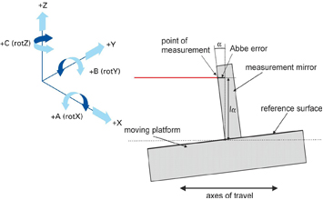
Image: Physik Instrumente (PI)

Minimizing Abbe error

Three approaches reduce Abbe error:

1. Reduce the Abbe offset. Mount the encoder as close as possible to the functional axis. In microscopy, this means placing the encoder at the focal plane height. In machining, it means measuring at the tool point.

2. Reduce the angular error. Use high-quality bearings (air bearings have pitch errors of 0.5 to 2 microradians over 100 mm, compared to 5 to 20 microradians for cross-roller bearings).

3. Measure and correct the angular error. Use a dual-encoder configuration or an autocollimator to measure pitch and yaw in real time, then compute and subtract the Abbe error. This is common in metrology stages with sub-50 nm accuracy requirements.

For piezo stages using ultrasonic friction-drive motors, the motor-to-bearing interaction affects angular error. The preload force of the piezo motor, applied at a specific point on the carriage, creates a moment that changes the pitch angle depending on the drive state. This motor-induced angular error is typically 0.5 to 2 microradians and is consistent (repeatable), so it can be calibrated out.

Long-term stability versus short-term repeatability

Datasheet repeatability is measured over minutes or hours in a controlled environment. Real applications run for days, months, or years. The stage's ability to maintain its position calibration over extended periods (long-term stability) is a separate specification from short-term repeatability, and it is rarely reported on datasheets.

Sources of long-term drift

Several mechanisms cause the relationship between encoder position and true position to change over time:

• Encoder scale relaxation. Glass and ceramic encoder scales are bonded to the stage body with adhesive. Over months, stress relaxation in the adhesive allows the scale to shift by 10 to 100 nm relative to the stage body. The scale still reads correctly relative to itself, but its relationship to the machine coordinate frame changes.

• Bearing wear. Cross-roller and ball bearings exhibit wear that gradually changes the carriage's geometric relationship to the base. After 10,000 km of travel (which a high-throughput inspection tool accumulates in months), the bearing preload, straightness, and angular errors may differ measurably from the as-calibrated condition.

• Thermal cycling effects. Repeated heating and cooling of the stage structure causes creep in bolted joints and adhesive bonds. Over hundreds of thermal cycles, the stage geometry can shift by 50 to 500 nm.

• PZT aging (for piezo-driven stages). The thermal behaviour of PZT ceramics includes time-dependent aging that gradually changes the motor's force output and, indirectly, the friction-driven stage's position calibration.

Recalibration intervals

For applications requiring absolute accuracy below 500 nm, periodic recalibration against a reference standard (laser interferometer or calibrated artifact) is necessary. Typical recalibration intervals:

Application	Accuracy requirement	Typical recalibration interval
Semiconductor metrology	< 100 nm	Daily to weekly
Photomask writing	< 50 nm	Every 8 to 24 hours
Optical inspection	< 500 nm	Monthly
General precision assembly	< 2 µm	Annually

Automated self-calibration routines, where the stage measures a fixed reference artifact at the start of each shift or lot, can maintain accuracy without operator intervention. This approach is standard in semiconductor tools and is increasingly adopted in other high-precision industries.

Multi-axis error interactions

Real stages have 6 degrees of freedom: X, Y, Z translation and rotation about each axis (roll, pitch, yaw). The datasheet specifications for positioning accuracy and repeatability refer only to the controlled axis, but errors in the other 5 axes affect the achieved accuracy at the point of interest.

Crosstalk and parasitic motion

When a single-axis stage moves in X, it also exhibits parasitic motion in Y and Z (straightness errors) and parasitic rotations (roll, pitch, yaw). These parasitic motions are caused by bearing imperfections, guide rail straightness, and motor-generated moments.

For a typical cross-roller bearing stage with 100 mm travel:

Error type	Typical magnitude
Straightness (Y deviation over X travel)	0.5 to 5 µm
Flatness (Z deviation over X travel)	0.5 to 5 µm
Pitch	5 to 50 µrad
Yaw	2 to 20 µrad
Roll	2 to 20 µrad

For an air bearing stage with 100 mm travel:

Error type	Typical magnitude
Straightness	0.05 to 0.5 µm
Flatness	0.05 to 0.5 µm
Pitch	0.5 to 5 µrad
Yaw	0.2 to 2 µrad
Roll	0.2 to 2 µrad

XY stage stacking errors

When two single-axis stages are stacked to form an XY system, the errors compound. The upper stage (carrying the workpiece) inherits all the geometric errors of the lower stage, amplified by the Abbe offsets between stages. A 200 mm XY stage built from cross-roller bearing stages typically achieves 2 to 10 µm XY planar accuracy (uncalibrated). After full error mapping with 21-point calibration on each axis, this reduces to 0.5 to 2 µm.

Monolithic XY stages (where both axes share a common base and guiding system) eliminate some stacking errors and typically achieve 2x to 5x better planar accuracy than stacked configurations. Air bearing XY stages achieve the best performance: 0.1 to 1 µm planar accuracy after calibration.

Practical advice for specification review

When evaluating datasheets, keep these guidelines in mind:

1. Ask how repeatability was measured. Unidirectional or bidirectional? How many cycles? What was the thermal environment? A number reported from 5 cycles in a temperature-controlled lab is more optimistic than the stage will deliver in a factory environment over thousands of cycles.

2. Ask what "accuracy" includes. Is it the systematic deviation only, or does it include the repeatability scatter (bidirectional accuracy per ISO 230-2)? The latter is a more honest number.

3. Check the calibration conditions. If the accuracy specification assumes laser-interferometer calibration at 20.0 °C, that accuracy is only valid under those conditions. Ask what the uncalibrated accuracy is; this tells you how much the stage relies on software correction versus mechanical precision.

4. Request the full accuracy plot. A single "accuracy" number (e.g., ±0.5 µm over 100 mm) hides the shape of the error curve. Some stages have a smooth, slowly varying error that is easy to calibrate out. Others have sharp, high-frequency errors from encoder interpolation that are difficult to correct and reappear as residual accuracy error.

5. Consider the application's thermal environment. If your process generates heat (laser processing, high-speed scanning friction), the stage's in-situ accuracy will be worse than the datasheet specification measured in a stable lab.

6. Bidirectional matters. If your application requires bidirectional positioning, do not accept a unidirectional repeatability specification as representative of your system's performance.

Summary

Repeatability and absolute accuracy are complementary, not interchangeable. Repeatability describes scatter; accuracy describes systematic offset. The encoder dominates repeatability; calibration and thermal management dominate absolute accuracy. Before selecting a stage, determine which specification your application actually requires, then allocate your budget accordingly. A stage that is overspecified in accuracy but adequate in repeatability may cost far more than the reverse, with no benefit to your process.