Applications / Optics & Photonics
Fiber alignment stages: achieving and holding sub-micron registration
The precision motion requirements for single-mode fiber coupling, from initial alignment search to long-term stability
Fiber Alignment Stages: Achieving and Holding Sub-Micron Registration
Coupling light into a single-mode optical fiber demands positioning accuracy that pushes against the limits of mechanical motion systems. A single-mode fiber at 1550 nm wavelength has a mode field diameter (MFD) of approximately 10 micrometers. To achieve 90% coupling efficiency, the fiber must be aligned to within 0.8 micrometers of the optimal position in all three axes. To reach 99% coupling, the tolerance shrinks to 0.25 micrometers. These submicron alignment tolerances (see repeatability vs. accuracy) must not only be achieved during initial alignment but maintained over hours, days, or years of operation, despite thermal drift, mechanical creep, and environmental vibration.
Piezoelectric actuators are the dominant technology for high-performance fiber alignment stages. This article examines why, covering the coupling physics that define the positioning requirements, the alignment algorithms that find the optimum, the stability challenges that threaten it (including thermal drift), and the multi-axis stage architectures that make it practical.
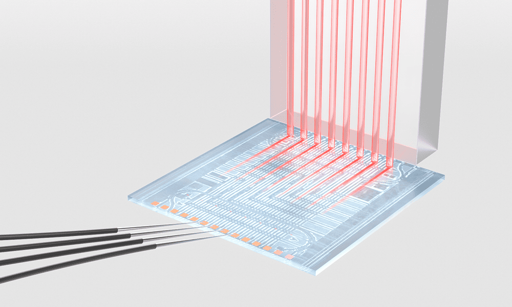
Image: Physik Instrumente (PI)
Single-Mode Fiber Coupling Requirements
Coupling Efficiency vs. Misalignment
The coupling efficiency between a Gaussian beam and a single-mode fiber is described by the overlap integral of the incident field with the fiber mode. For a Gaussian beam focused to a spot matching the fiber mode, the coupling efficiency as a function of lateral misalignment delta_x is:
eta = exp(-2 * delta_x^2 / w^2)
where w is the mode field radius (MFD/2). For MFD = 10.4 micrometers (standard SMF-28 at 1550 nm), w = 5.2 micrometers:
| Lateral misalignment | Coupling efficiency | Loss (dB) |
|---|---|---|
| 0 | 100% | 0 |
| 0.5 um | 96.3% | 0.16 |
| 1.0 um | 85.9% | 0.66 |
| 1.5 um | 70.6% | 1.51 |
| 2.0 um | 53.8% | 2.69 |
| 2.6 um (1/e^2 radius) | 36.8% | 4.34 |
| 5.2 um (mode radius) | 1.8% | 17.4 |
The exponential dependence makes the alignment exquisitely sensitive. A 1 micrometer misalignment costs 0.66 dB. A 2 micrometer misalignment costs 2.69 dB. For telecom applications where the total link budget is 20 to 30 dB and every 0.1 dB matters, alignment tolerances of 0.3 to 0.5 micrometers are mandatory.
Axial (Focus) Alignment
Axial misalignment (along the beam propagation direction) affects coupling through defocus. For a Gaussian beam focused by a lens with focal length f and NA = sin(theta):
The axial tolerance is approximately:
delta_z (for 1 dB loss) = +/- n * lambda / (pi * NA^2)
For NA = 0.15 (a typical fiber coupling lens) at 1550 nm:
delta_z = +/- 1 * 1.55 / (pi * 0.0225) = +/- 21.9 micrometers
The axial tolerance is roughly 20x larger than the lateral tolerance because defocus produces a quadratic (not exponential) coupling loss. This asymmetry has implications for stage design: the Z axis needs more travel but less resolution than the X and Y axes.
Angular Alignment
Tilt of the fiber or the beam relative to the optimal axis also reduces coupling. The angular tolerance for 1 dB loss is approximately:
delta_theta = lambda / (pi * w) = 1.55 / (pi * 5.2) = 95 milliradians = 5.4 degrees
This relatively large angular tolerance means that angular alignment is typically not the critical parameter for single-fiber coupling. However, for fiber arrays (where multiple fibers must be simultaneously aligned), angular errors accumulate across the array and become significant.
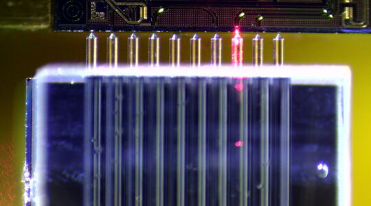
Image: SmarAct GmbH
Alignment Algorithms
Finding the position that maximizes coupling efficiency requires a search algorithm. The alignment stage must move the fiber through a search pattern while monitoring the coupled power. Several algorithms are used, with different tradeoffs between speed, robustness, and convergence accuracy.
Raster Scan
The simplest approach: scan the fiber across a grid pattern (typically in X and Y) while recording the coupled power at each point. The position with maximum power is the alignment optimum.
Advantages: simple, guaranteed to find the global optimum if the grid is fine enough and the search area covers the optimum. Disadvantages: slow. For a 50 x 50 micrometer search area with 0.5 micrometer grid spacing, the grid has 100 x 100 = 10,000 points. At 1 ms per point (limited by detector integration time), the scan takes 10 seconds. Finer grids or larger search areas are proportionally slower.
Piezo stages are well-suited for raster scanning because they offer smooth, continuous motion with nanometer-level repeatability. The absence of backlash (unlike screw-driven stages) ensures that the measured power map is accurate and reproducible.
Gradient Search (Hill Climbing)
Starting from an initial position, the algorithm evaluates the coupled power, then takes a small step in the direction that increases power. This process repeats until the power stops increasing (the gradient approaches zero).
Common gradient methods include:
Simplex (Nelder-Mead): Uses a triangle of three test points (in 2D) to determine the search direction. Robust against noise and does not require derivative computation. Converges in 30 to 100 steps for a well-shaped coupling peak.
Dithering gradient: The stage oscillates (dithers) in X and Y at a known frequency. The resulting power modulation is demodulated (using a lock-in amplifier or synchronous detection) to extract the gradient. The stage moves in the gradient direction at a rate proportional to the gradient magnitude. This method provides continuous, real-time gradient information and is the basis for active alignment (continuous tracking of the optimum).
Spiral search: The stage traces an outward spiral from the initial position. When the power exceeds a threshold, the algorithm switches to a finer spiral or a gradient search to converge on the peak. This approach is efficient when the initial position is uncertain.
For piezo stages, the dithering gradient method is particularly effective because:
- Piezo stages can dither at frequencies of 100 Hz to 10 kHz with nanometer amplitudes, far above the mechanical resonance of most fiber assemblies.
- The dither does not introduce significant coupling loss because the dither amplitude (10 to 100 nm) is small compared to the mode field diameter.
- Synchronous detection achieves high signal-to-noise ratio even with low coupled power levels.
Convergence Time Comparison
For a typical single-fiber alignment starting 25 micrometers from the optimum:
| Algorithm | Typical convergence time | Final alignment accuracy |
|---|---|---|
| Raster scan (0.5 um grid) | 5 to 15 seconds | 0.25 um (grid limited) |
| Simplex | 0.5 to 2 seconds | 0.1 um |
| Dithering gradient | 0.1 to 0.5 seconds | 0.05 um |
| Spiral + gradient | 0.5 to 3 seconds | 0.1 um |
The dithering gradient method achieves the fastest convergence and finest accuracy, making it the preferred choice for production alignment systems. Its real-time gradient tracking also enables automatic re-alignment if the coupling degrades during operation.
Thermal Drift and Long-Term Stability
Achieving sub-micron alignment is the easy part. Maintaining it is the hard part. Thermal drift is the dominant source of long-term alignment degradation in fiber-coupled systems.
Sources of Thermal Drift
Differential thermal expansion: The fiber, the lens, the laser or waveguide chip, and the mounting structure all have different coefficients of thermal expansion (CTE). A 1 degree Celsius temperature change produces differential expansion that depends on the material pair and the distance between the components.
For a typical fiber-to-chip coupling assembly with a 10 mm path length between the fiber and the chip, using an aluminum submount (CTE = 23 ppm/K) and an InP chip (CTE = 4.6 ppm/K):
Differential expansion per degree: (23 - 4.6) * 10^-6 * 10 mm = 0.184 micrometers/K
A 5 degree Celsius temperature change produces 0.92 micrometers of drift, enough to reduce coupling from 100% to below 86% (0.66 dB loss). Over a 50 degree Celsius operating range (-10 to +40 degrees Celsius), the total drift is 9.2 micrometers, more than the entire fiber mode field diameter.
Solder and adhesive creep: Epoxy adhesives and solder joints used to fix the fiber in place undergo creep (slow plastic deformation under stress). The creep rate depends on the stress level, temperature, and material. UV-cured epoxies typically creep 0.1 to 1 micrometer over the first year, with a logarithmic time dependence. Low-shrinkage epoxies and laser-welded joints have lower creep rates (10 to 100 nm per year).
Component aging: Laser diode output beam characteristics can change with aging (due to facet degradation or waveguide changes), shifting the optimal fiber position. Fiber Bragg gratings and other in-fiber components can also shift with temperature and aging.
Passive Stability Strategies
Material matching: Using mounting materials with CTEs matched to the active component (InP, GaAs, or silicon) minimizes differential expansion. Common choices include Kovar (CTE = 5.1 ppm/K for InP), Invar (CTE = 1.2 ppm/K for silicon), and aluminum nitride (CTE = 4.5 ppm/K for InP).
Athermal design: Arranging the geometry so that thermal expansions cancel at the fiber tip. For example, if the fiber is mounted in a tube that expands in the opposite direction to the submount expansion, the net displacement at the fiber tip can be zero. This requires careful geometric design and precise CTE characterization.
Laser welding: Instead of adhesive bonding, the fiber ferrule is welded to the mounting clip using a YAG laser. Laser welding produces a metallurgical joint with zero creep and sub-100 nm alignment shift during the welding process. The fiber is held by the piezo stage during welding and released after the weld cures. This technique is standard in telecom transceiver manufacturing.
Active Alignment and Tracking
For applications where passive stability is insufficient (long-haul telecom amplifiers, free-space receivers, experimental setups), active alignment uses the piezo stage to continuously track the optimum coupling position.
The dithering gradient algorithm described earlier runs continuously, adjusting the fiber position to maintain maximum coupling. The dither amplitude (typically 50 to 200 nm) produces a negligible coupling loss (below 0.01 dB for 100 nm dither on a 10 micrometer MFD fiber) while providing continuous gradient information.
Active alignment with a piezo stage can maintain coupling to within 0.05 micrometers of the optimum indefinitely, compensating for thermal drift, creep, and vibration. The bandwidth of the tracking loop is typically 1 to 100 Hz, sufficient to track thermal changes (millihertz to sub-hertz) and low-frequency vibration.
The cost of active alignment is complexity: the system requires a power monitor, a controller, and a piezo stage with power continuously applied. Piezo creep under sustained voltage can be a concern, but closed-loop stages with capacitive sensors eliminate this issue.
Multi-Axis Alignment Stage Architectures
Fiber alignment requires motion in at least three axes (X, Y, Z) and sometimes five or six axes (adding Rx, Ry, Rz for angular alignment). The stage architecture determines the alignment speed, accuracy, and stability.
Stacked Linear Stages
The simplest architecture stacks three independent linear stages (X on the bottom, Y in the middle, Z on top). Each stage has its own piezo actuator and flexure.
Advantages: simple design, straightforward control (independent axes). Disadvantages: stacking errors accumulate. The Z stage (on top) has the largest parasitic motion because it moves with both the X and Y stages. The total moving mass for the Z stage includes the Y and Z stages plus the fiber holder, which reduces the Z-axis resonance frequency and bandwidth.
Abbe errors (angular errors causing position errors at a distance from the stage) are significant for stacked stages. A 10 microradian angular error in the X stage produces a 10 microradian * 30 mm = 0.3 micrometer position error at the fiber tip (30 mm above the X stage), which is comparable to the alignment tolerance. Minimizing Abbe errors requires placing the fiber tip as close to the motion axes as possible.
Parallel Kinematic Stages
In a parallel kinematic architecture, all actuators connect directly between the base and the moving platform. A flexure-based hexapod (Stewart platform) with six piezo actuators provides six-axis motion with no stacking.
Advantages: all axes have equal dynamic performance (no stacking penalty). Abbe errors are minimized because all actuators act on the same platform. The moving mass includes only the platform and fiber holder (no intermediate stages). Disadvantages: coupled kinematics. Driving the platform in X requires coordinated motion of all six actuators. The controller must compute the inverse kinematics for each command. Cross-coupling between axes requires calibration.
For fiber alignment, a three-axis parallel kinematic stage (using three piezo actuators in a tripod configuration) provides X, Y, and Z motion with a compact form factor. The actuators are arranged at 120-degree intervals and coupled to the platform through flexure joints. The inverse kinematics is straightforward, and the cross-coupling is minimal for small displacements.
Hybrid Architectures
Some designs use a coarse stage (stepper motor or DC motor with lead screw) for initial approach (millimeters of travel) and a fine piezo stage for final alignment (tens of micrometers of travel). This hybrid approach combines the long travel range of electromagnetic motors with the sub-micron accuracy of piezo actuators.
The coarse stage brings the fiber to within the capture range of the fine stage (typically 20 to 100 micrometers). The fine stage then performs the precision alignment. After alignment, the coarse stage is locked (power off, brake engaged), and the fine stage maintains the alignment.
For production fiber alignment (transceiver assembly), the coarse-fine hybrid is standard. The coarse stage positions the fiber to within 5 to 10 micrometers using machine vision (camera viewing the fiber and the chip), and the fine piezo stage completes the alignment using power monitoring.
Piezo Actuator Selection for Fiber Alignment
Travel Range Requirements
The fine stage travel range must accommodate:
- The coarse stage positioning error (5 to 20 micrometers).
- The thermal drift range over the alignment and bonding process (1 to 5 micrometers for a 10-minute process with 2 degree Celsius temperature variation).
- Servo headroom (20% to 50% of the total range reserved for control margin).
A total travel range of 30 to 100 micrometers per axis is typical for fine alignment stages. This is well within the range of multilayer piezo stacks (which produce 10 to 100 micrometers of travel depending on stack length and voltage).
Resolution Requirements
The alignment resolution must be 5x to 10x better than the alignment tolerance. For a 0.3 micrometer alignment tolerance, the resolution must be 30 to 60 nm. Piezo stacks with closed-loop capacitive sensors easily achieve 1 to 10 nm resolution, providing 10x to 100x margin.
Bandwidth Requirements
The bandwidth requirement depends on the alignment algorithm:
- Raster scan at 10 mm/s: the stage traverses 100 micrometers in 10 ms, requiring a bandwidth of approximately 100 Hz.
- Dithering gradient at 1 kHz dither frequency: the stage must respond at 1 kHz with amplitudes of 50 to 200 nm. This requires a bandwidth of at least 1 kHz.
- Active tracking at 100 Hz: the stage must respond at 100 Hz with amplitudes of up to 1 micrometer. This requires a bandwidth of at least 100 Hz.
Piezo stack stages with flexure guidance achieve bandwidths of 500 Hz to 5 kHz depending on the moving mass. This comfortably exceeds the requirements for all common alignment algorithms.
Comparison with Motorized Stages
Motorized stages (stepper motor or DC servo with lead screw or ball screw) are the low-cost alternative to piezo stages for fiber alignment. Their limitations for precision alignment include:
Backlash: Lead screws have backlash of 1 to 10 micrometers. Ball screws have 0.1 to 1 micrometer backlash. Preloaded ball screws reduce backlash to below 0.1 micrometer but increase friction and cost. Backlash makes bidirectional alignment unreliable and slows convergence of gradient algorithms.
Friction: Static friction (stiction) in screw-driven stages causes stick-slip motion with minimum incremental motion of 50 to 500 nm. This limits the alignment accuracy to the stiction level. Piezo stages with flexure guidance have zero stiction.
Speed: Stepper motors with lead screws have slow step-settle characteristics (1 to 10 ms per step at micrometer resolution). A 10,000-point raster scan takes 10 to 100 seconds. Piezo stages complete the same scan in 1 to 10 seconds.
Stability: Stepper motors can hold position without power (the detent torque of the stepper and the friction of the lead screw prevent backdriving). This is an advantage over piezo stages that require continuous power for position holding (unless the stage has a mechanical lock).
For production alignment where cost and throughput are both critical, some systems use motorized stages with encoder feedback for the coarse search and switch to piezo fine stages for the final convergence. This approach achieves alignment times of 1 to 3 seconds per fiber, compared to 0.5 to 1 second for an all-piezo system.
Practical Performance Numbers
Single-Fiber Alignment
| Parameter | Typical production system | High-performance lab system |
|---|---|---|
| Alignment axes | 5 (X, Y, Z, Rx, Ry) | 6 (X, Y, Z, Rx, Ry, Rz) |
| Fine stage travel | 100 um per axis | 200 um per axis |
| Fine stage resolution | 5 nm | 1 nm |
| Alignment time (to within 0.3 um) | 0.5 to 2 seconds | 0.1 to 0.5 seconds |
| Achieved coupling efficiency | 80% to 95% (-1 to -0.2 dB) | 95% to 99% (-0.2 to -0.04 dB) |
| Passive stability (after bonding) | 0.5 to 2 um drift over 24 hours | N/A (actively tracked) |
| Active tracking stability | N/A | <0.05 um indefinitely |
| Throughput | 300 to 1000 alignments/hour | N/A (research use) |
Fiber Array Alignment
Fiber arrays (V-groove arrays of 4 to 64 fibers) are aligned to photonic integrated circuits (PICs) or laser arrays. The alignment challenge is to simultaneously optimize coupling for all fibers, which requires higher-DOF stages and more sophisticated algorithms.
| Parameter | V-groove array alignment |
|---|---|
| Number of fibers | 4 to 64 |
| Pitch | 127 or 250 micrometers |
| Alignment DOF | 6 (X, Y, Z, Rx, Ry, Rz) |
| Critical tolerance | Rotation (Rz): 10 to 50 microradians |
| Typical coupling efficiency | 70% to 90% average across array |
| Alignment time | 5 to 30 seconds |
Array alignment is more demanding than single-fiber alignment because rotational errors (Rz) couple into lateral misalignment across the array. A 50 microradian Rz error produces 50 * 10^-6 * 8 mm = 0.4 micrometer lateral error at the edge of a 16-fiber array (at 250 micrometer pitch), which exceeds the single-fiber tolerance. This is why array alignment stages must provide rotational control with microradian accuracy.
UV-Curing and Laser Welding with Piezo Stages
The final step in fiber alignment is fixing the fiber in place. The piezo stage holds the fiber at the optimal position while an adhesive is cured or a weld is formed.
UV Epoxy Curing
UV-curable epoxy is applied between the fiber and the mounting surface. UV light (365 to 405 nm) is then applied to cure the epoxy. During curing, the epoxy shrinks by 1% to 5%, which translates into 0.5 to 5 micrometers of fiber displacement for a typical bond line thickness of 50 to 100 micrometers.
The piezo stage must compensate for this shrinkage in real time. Active alignment during UV curing tracks the coupling peak as the epoxy contracts, adjusting the fiber position to maintain maximum coupling. After the epoxy is fully cured (typically 10 to 30 seconds), the piezo releases and the fiber is held by the epoxy.
The post-cure alignment shift depends on the residual stress in the epoxy and its creep characteristics. Low-shrinkage epoxies (below 1% volumetric shrinkage) and staged curing protocols (partial cure, relax, full cure) minimize the post-release shift to below 0.5 micrometers.
Laser Welding
Laser welding (using a pulsed Nd:YAG laser at 1064 nm) melts a small spot on the fiber mounting clip, deforming it to shift the fiber position. Multiple welds at different locations can bring the fiber to the optimal position and fix it in place.
The piezo stage serves a different role in laser welding. Rather than holding the fiber during a bonding process, the stage provides a reference measurement of the optimal position. The alignment algorithm finds the optimum using the piezo stage, records the optimal position, and then the laser welding system applies welds to shift the mechanical structure to match that position.
After each weld, the fiber position shifts by 0.1 to 2 micrometers (depending on the weld energy and location). The piezo stage measures the new position, and the next weld is planned to reduce the remaining error. After 5 to 20 welds, the alignment is typically within 0.3 micrometers of the target.
Laser welding produces joints with zero creep and superior long-term stability compared to epoxy bonding. The alignment shift during welding is compensated by the multi-weld approach, and the final alignment accuracy depends on the accuracy of the position measurement (piezo stage + sensor) and the weld-by-weld correction algorithm.
Emerging Challenges
Silicon Photonics
Silicon photonic devices have smaller mode fields than standard single-mode fiber (MFD of 3 to 5 micrometers for a silicon waveguide, compared to 10 micrometers for SMF-28). This tightens the lateral alignment tolerance by 2x to 3x, requiring sub-0.1 micrometer alignment accuracy.
Edge couplers with spot-size converters expand the mode field to 5 to 10 micrometers, relaxing the tolerance back to levels compatible with current piezo stage technology. However, as integration density increases and spot-size converters become impractical for some designs, the alignment requirements will push toward 50 nm accuracy, requiring improved stage resolution and thermal stability.
Multi-Channel Alignment
Co-packaged optics for data center switches require alignment of 32 to 128 fiber channels simultaneously. The alignment time per channel must be minimized to achieve production throughputs of 100+ assemblies per hour. Parallel alignment of multiple fibers using array stages (with independent piezo actuation per fiber) is an active area of development.
Cryogenic Fiber Alignment
Quantum computing and superconducting detector systems require fiber-coupled optical links at cryogenic temperatures (4 K or below). The thermal contraction from room temperature to 4 K is 3 to 5 mm for common materials (aluminum, copper), producing enormous differential displacements. Standard piezo actuators lose 80% to 90% of their displacement at 4 K (due to the temperature dependence of the piezo d33 coefficient), though they remain functional. Specialized cryogenic alignment stages with PZT optimized for low-temperature operation are an active research area.
Summary
Fiber alignment is one of the most demanding applications for precision motion stages, combining sub-micron positioning accuracy with the requirement for long-term stability under thermal, mechanical, and chemical stresses. Piezoelectric stages dominate this application because they provide the resolution (nanometers), bandwidth (kilohertz), and zero-friction motion needed for fast, accurate, and repeatable alignment. The choice between open-loop and closed-loop operation, the alignment algorithm, the bonding method, and the thermal management strategy all affect the final coupling efficiency and stability. As photonic systems push toward smaller mode fields and higher channel counts, the demands on fiber alignment stages will continue to intensify, keeping piezoelectric actuation at the center of the technology.